Your Questions Answered #5 – Tips and Tricks Live extended: What is your favourite underappreciated formula?

• 'Excel tips and tricks live – your questions answered (June 2023)' webinar recording now available.

The question

What is your favourite underappreciated formula?

Answer

For me it's probably HYPERLINK. By using a combination of the CELL and HYPERLINK functions it's possible to create a clickable link to anywhere in a workbook, and the link will follow the target cell even when new rows or columns are added.

This is the complete formula you'd need, and below I'll explain how to use it and how it works.

=HYPERLINK("#"&CELL("address",target_cell),link_text)

For example, let's say we have a financial model and we wanted to include a link from the output P&L to the Revenue inputs which start at cell F44 on sheet Sheet1. We could use this formula to make a clickable link:

=HYPERLINK("#"&CELL("address",Sheet1!F44),"Revenue Inputs")

The Sheet1!F44 part is a link to the cell which we want to hyperlink to, and the function CELL(info_type, reference) can be used to return the address of that target. In this instance we want to get the "address" info type, and the target is going to be cell F44 on Sheet1. This function evaluates to [Book1]Sheet1!$F$44, where Book1 is the workbook name. The great thing about this is that because the reference cell is a link, that target will "follow" that cell around when new rows/columns are inserted.

We can then pass that dynamic address to the HYPERLINK function as the link_location, by prefixing it with the # sign. And then finally we can give the link a name, which is what will appear to the user so they know where the link will take them, in this case I've hardcoded it as "Revenue Inputs" but that could be linked to the title of the revenue section if you wanted, or even to the target cell Sheet1!F44 if that was the title for the inputs section.

I know everyone loves the INDEX/MATCH combination, but I think that HYPERLINK/CELL is probably my favourite underappreciated formula because it's "easy when you know how" and it builds really robust hyperlinks which aid navigation and automatically stay up to date.

The question

Data grouping: How can I extend range without "ungrouping" first and then "re-grouping" the range?

Answer

The simple answer to this is that the rows to be grouped (or columns – but this answer will focus on rows) can be selected, click on the Data tab on the ribbon then click on the Group button and the rows will have their outline level updated. The rows won't automatically be shown/hidden until you click on one of the controls; either the numbers above the outline grouping levels, or the [+] or [-] icons next to the grouped rows.

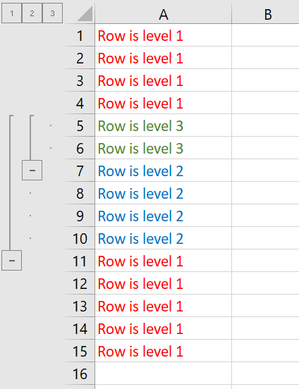
To explain in a bit more detail, each row has an assigned "outline level", this is not shown until some rows are grouped. The default level for ungrouped rows is level 1. When rows are "grouped" they will have their outline level increased to 2, and this can be seen by the position of the dots which are under the '2' at the top.

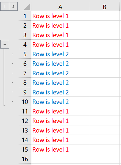
The [-] button next to row 11 will hide rows 5-10. They could also be hidden by clicking on the number '1' at the top left. (By the way, if we wanted to add rows 3 and 4, I could simply highlight those rows and click on 'Data' > 'Group'.)

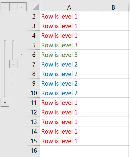
What's interesting is that rows can be grouped with various different levels, to create further sub-levels. Say we wanted to hide rows 5-6 at a deeper level, we could highlight those two rows and click on 'Data' > 'Group':

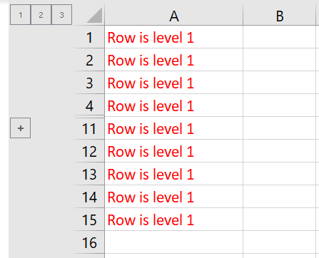
This becomes really helpful when we click on the 1, 2 and 3 at the top, as these will define the level of detail which is shown. For example, clicking on 1 shows only rows with level 1:

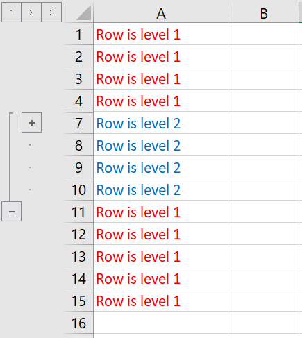
We could also click on 2 to show rows with level 2 or lower (ie, levels 2 and 1):

And finally, we can click on the 3 to show rows with level 3 or lower (ie, in this case levels 3, 2 and 1):

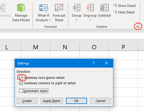
The final tip I would like to include here is that you can move the outline grouping buttons to the top of each section. To do this click on Data tab, then on the little square in the bottom right of the Outline tools group and then untick the "Summary Rows Below Detail".

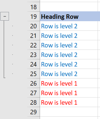
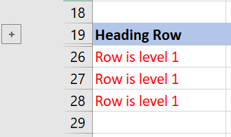
The buttons will work the same, but now the [+] and [-] buttons are shown above the grouping ranges. This can be helpful if you have a header row and then you want to hide the details of a section below:

The question

What does pasting constants do?

Answer

Great question, this was covered on the webinar, but this is a good opportunity to recap the pastespecial options.

The simple answer is that it pastes the current values of the cells only, without the formulae. It's a way to convert formulae into their values and freezes them as they were at the point they were copied.

To provide a bit more info on how / why you might want to do this let me expand. Once an area has been selected and you click COPY or press CTRL+C to copy it goes onto your clipboard. Sometimes you will want to paste everything, in which case you can press CTRL+V or simply click the default Paste option. This might be what you want but be aware that it can sometimes have unintended consequences; when pasting formulae any "non-locked" parts of the formulae references will move, ie, anything not locked with a dollar sign $ will be a relative reference and will move and the formulae might not do what you wanted as a result. There's also a number of other properties of a copied area which you may or may not want, things like styles, named ranges referenced, conditional formatting, font style, number format, cell validation and a range of other properties. Simply copying and pasting will recreate everything about the source cells, and this can start to get messy, especially when copying from one workbook to another.

I'd recommend, if you only actually want to paste the values, then just past the values! This can be done by pressing ALT+E, then S, then V or right clicking and selecting Paste Special from the paste menu. You can then choose 'values' to paste only the values which were copied. Other options in there are to paste other specific components of the source range, like just the formulae (with no formatting), or just the formatting (with no formulae or values) or just the cell validation etc. Using this menu provides a lot of flexibility and enables you to keep your workbooks a bit cleaner and tidier by avoiding coping things you didn't mean to! Excel Online now also supports the keyboard shortcut Ctrl+Shift+V to paste values (a shortcut that users of other applications may already be familiar with).