Simple but effective, part 2: extending Tables

Excel Tables – so much more than just a pretty format

When Tables were first introduced into the Windows versions of Excel in Excel 2007, many people saw them as another Excel formatting ‘gimmick’. This view was supported by the inclusion of the Format as Table command in the Styles group of the Excel Home Ribbon tab. However, it soon became apparent that Tables were much more important than that, and that they had a significant role to play in many aspects of automating Excel.

Having looked at different methods of turning ranges of cells into Tables in part 1, in this part, we will see in more detail what happens when we add data, or formulas, to cells in rows and columns adjacent to our existing Table.

Extending a Table - rows

Last time, we used a high-profile spreadsheet ‘horror story’ to show how using Tables could help prevent a common type of error. We’ll start this time by demonstrating how this works. Here we have a simple price list. In columns A and B we have just entered the data in a contiguous block of cells. In columns D and E, we have the same data, but this time we have turned the block of cells into an Excel Table. Above each of our price lists, we have included formulas that use the SUM() function to calculate the total of our price list values. For our Table, we have entered this formula in two different ways. In E2, we have just copied the formula from B2 so that it uses normal cell references. In cell E3, we have dragged over our three cells in the Table to create our SUM() range. This automatically uses a structured ‘Table language’ that refers to the name of the Table and the column heading:

tblPrices[Price]

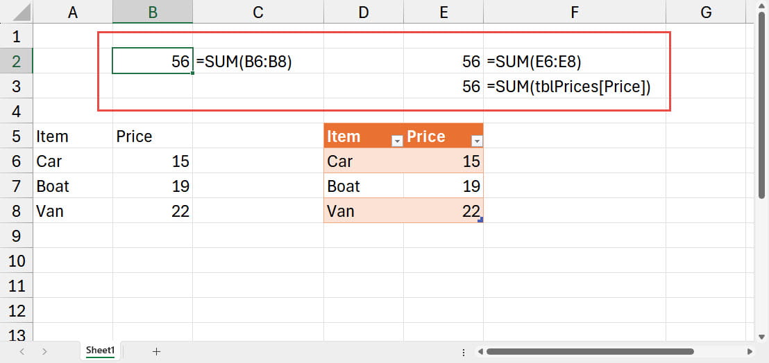
This structured language makes it much clearer that we are trying to refer to the whole column and, as long as we use descriptive names for our Tables and Table columns, helps to create formulas that should make it much easier for the user to understand. Note that we can change the Table name from the default ‘Table’ by clicking any cell in the Table to display the contextual Table Design Ribbon tab. The Table Name text box can be found in the left-hand ‘Properties’ group of the tab. Using a consistent prefix such as tbl can be helpful in distinguishing Tables from other Excel objects and for finding them in the list of AutoComplete items when constructing a formula.

Let’s see what happens when we add another item to the cells immediately beneath our two price lists:

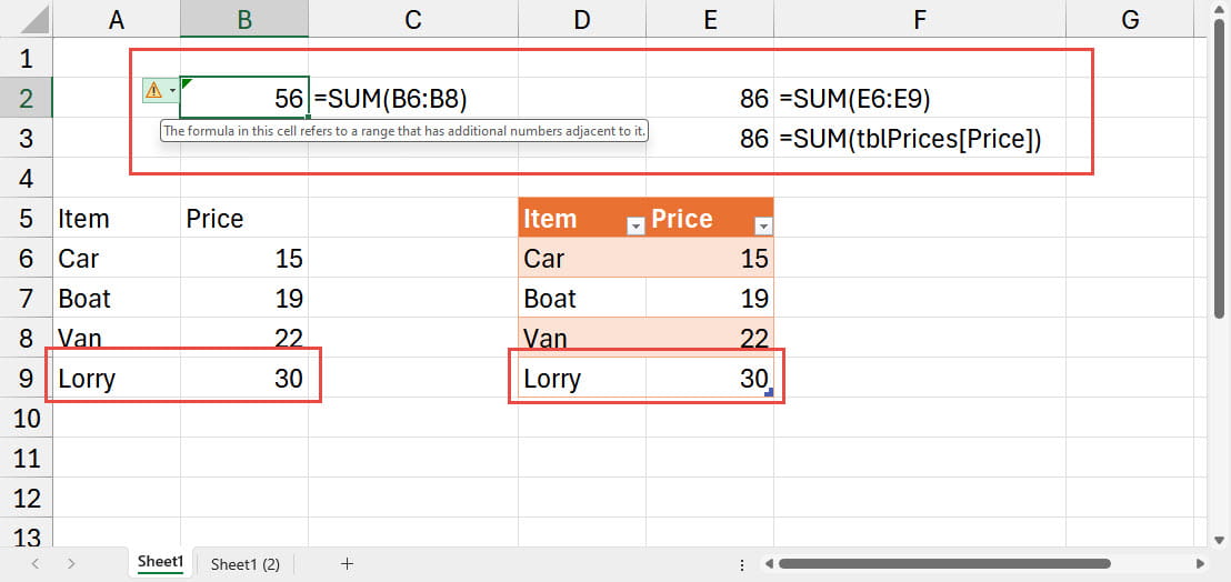
As you can see, for our simple range of cells, our SUM() formula does not adjust to our additional item in the list. Depending on your Excel Options, an error check message might appear to warn you that: “The formula in this cell refers to a range that has additional numbers adjacent to it” and clicking on the error dropdown will allow you to update your formula to include the relevant cell or cells. Looking at our Table example, adding data in the cells immediately below our Table causes the Table to expand automatically to include the added cells. Unsurprisingly, the SUM() formula in cell E3 that refers to the range of cells using the Table name and column heading now shows the correct total. However, our SUM() formula in cell E3, that just uses cell references, also adapts automatically to include our added item.

Extending a Table - columns

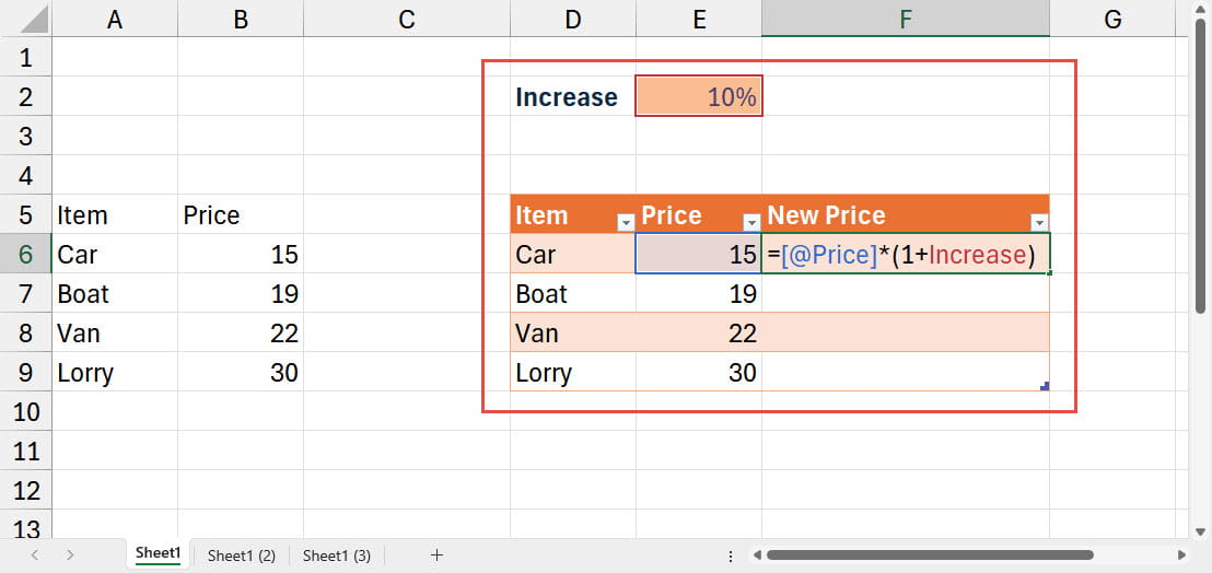
In order to demonstrate what happens when we add data to the cells immediately to the right of a Table, we have adapted our example to include a price increase value. We have used an Excel Range Name to allocate the name ‘Increase’ to this cell. When we type in our new column heading in cell F5, because it is adjacent to our existing Table, the Table expands to include the new column in the same way that it did to include the new row. We can then enter our formula by clicking on the cells that we want to use. The reference to the cell within the Table uses the structured Table language:

=[@Price]

There is no need to use the Table name as the cell is within the same Table, but we do need to be able to set the reference to use the same row, Excel does this by automatically using the @ operator.

Because we have given our price increase cell a Range Name, we can simply use the Range Name to refer to it without needing to worry about fixing our reference using the dollar signs:

=[@Price]*(1+Increase)

When we accept our new formula, not only will it calculate our value in cell F6, but it will also automatically fill our new formula down to the rest of the column:

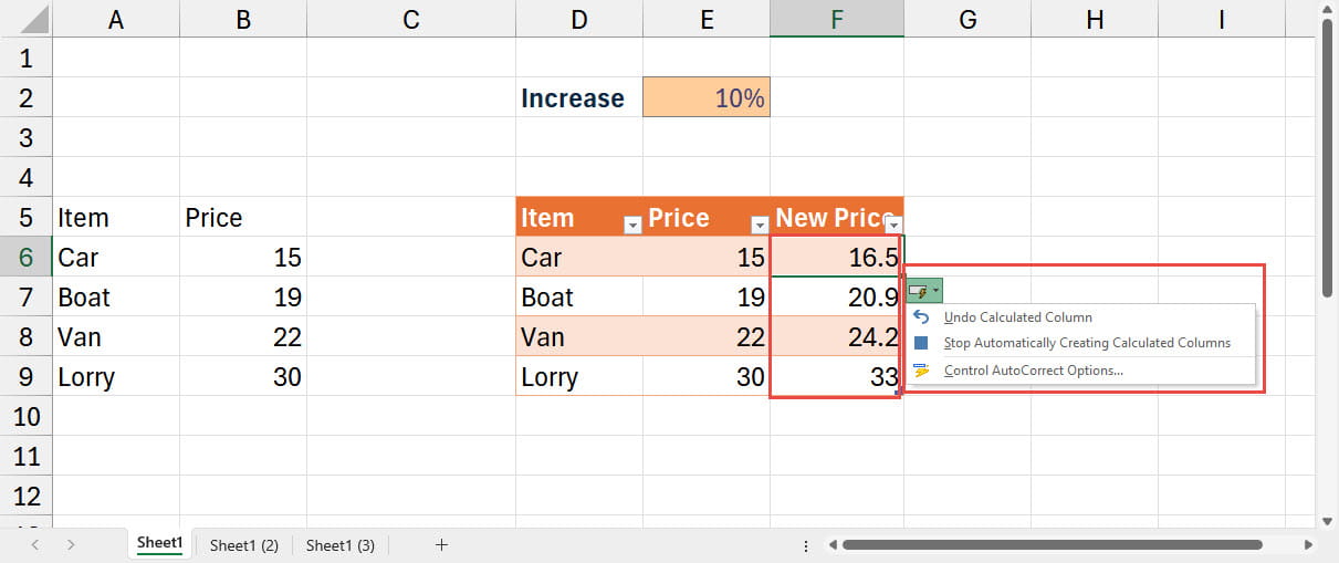
Note that an AutoCorrect Options prompt will appear that you can click on to choose to undo the automatic Calculated Column operation, or even to stop Excel from ‘Automatically Creating Calculated Columns’.

Extending a Table – formulas and formatting

Not only is the formula copied to all the existing rows in our Table, but if a column contains a consistent formula, as we add rows to our Table, that formula will also be automatically copied to those new rows.

As you can see above, there is no particular number formatting applied to our cells. Here, before adding our new Train row, we have set number formats for all the cells in each of our value columns and then added our new row item. As well as the formula, our formatting is also automatically copied to the new row:

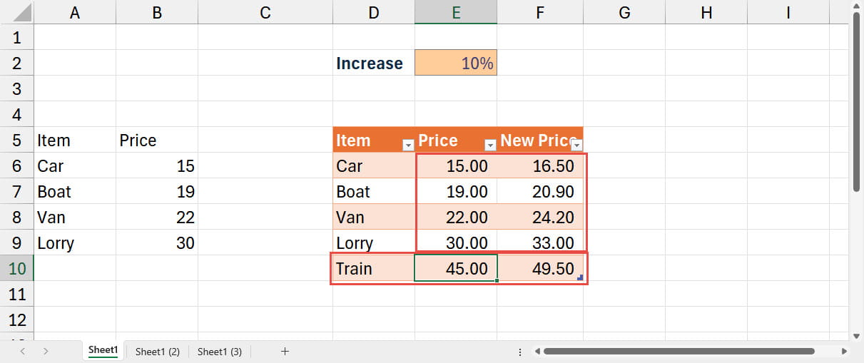
Although the copying of number formatting seems to work most of the time, I have noticed that occasionally, despite the formatting being consistent in the column, the number formatting is not copied correctly to new rows.

Next time…

In the next part of the series, we will see how to change the dimensions of a Table manually, before moving on to examine some of the practical benefits of Tables in general and calculated columns in particular.

Conclusion

You can explore Tables; Range Names and fixed references; Excel error checking and a great deal more, in the ICAEW archive:

• Browse the archive