
Hello all and welcome back to the Excel Tip of the Week! This week we have a Basic User post in which we’re taking a fresh look at the ins and outs of hidden rows and columns. This was first discussed in TOTW #192.
How and why to hide and unhide rows and columns
You can hide a selection of rows and columns simply by selecting the ones you want, right clicking, and clicking Hide:
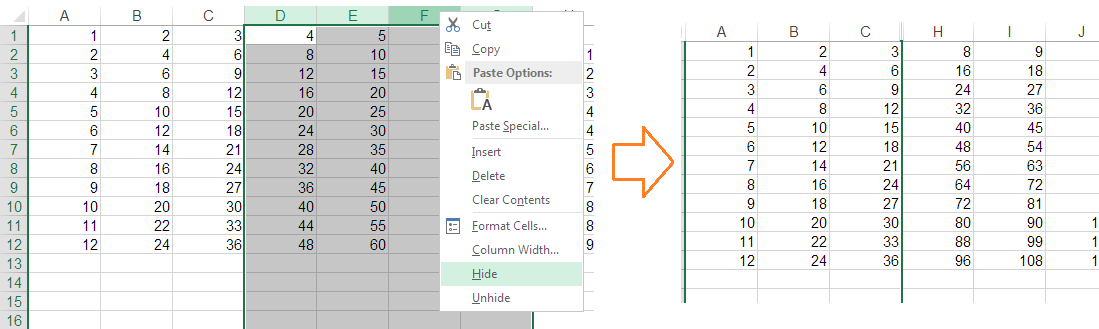
This doesn’t remove or change anything about the data in the cells that you hide – all it does is hide them. This means that any formulas in those cells will continue to update, and any formulas that refer to values in the hidden cells will still include them (with a couple of exceptions for specific formulas such as SUBTOTAL and AGGREGATE that specifically don’t behave this way). For the most part, hiding cells is purely aesthetic.
There is one use for hiding cells which is a little more practical – making a limited-size spreadsheet for easier navigation:
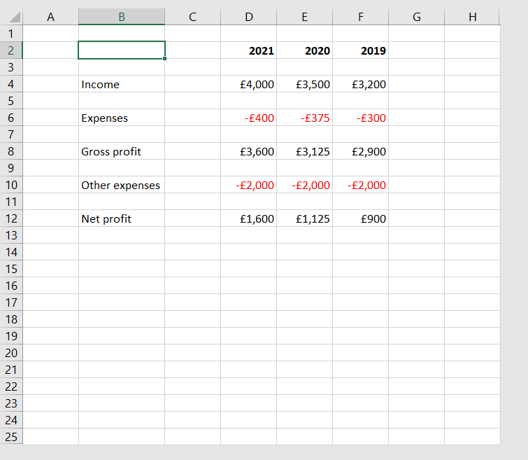
Here all rows and columns after 25 and H have been hidden. This means that the keyboard shortcuts Ctrl right-arrow and Ctrl down-arrow will navigate to the edges of the used area, instead of way out to column XFD or row 1,048,576 as usual. Although note that all those unused rows and columns still exist – they are only hidden from view.
Unhiding rows and columns is largely the same – just highlight a selection that includes the ones you want to unhide, right click the appropriate heading, and select Unhide. If appropriate, click the arrow symbol at the top-left of the cell grid to select the entire sheet before unhiding to reveal all the hidden cells.
Why hidden cells go wrong
As you can see from the above example, hidden rows or columns can be tricky to detect – you can tell because of the slightly thicker border between the C and H column headings (and of course the fact that the letters skip from C to H). But hidden cells are notoriously easy to miss. This can cause a variety of issues – for example, a reviewer might miss an interstitial calculation that’s been hidden for aesthetic reasons, or be unable to make sense of a formula result because some of the data it’s working with isn’t visible. This is of course particularly bad if the spreadsheet has been screen-capped or printed.
But the issues actually go deeper – hidden cells can lead to actual errors. For the most part, any cell operation you do on a range still includes any hidden cells within that range – such as deleting or copying. This means that e.g. copying a formula over a range with some hidden cells in it will automatically overwrite those cells – even if that’s not what you would have wanted. While you can use the Alt ; shortcut to select only the visible cells in a range, this is easy to forget or go wrong with.
But hiding intermediate calculations and other things for presentational purposes is a legitimate aim, so what to do? The answer is to use grouped rows and columns instead. These let you hide cells in much the same way, but with a much clearer marking that something is hidden, and an easier way to flip the visibility back and forth with +/- buttons. It even offers the ability to have multiple layers of visibility stacked within one another.
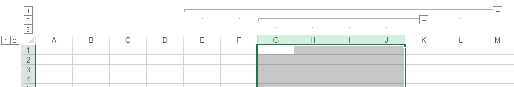
Find out more about grouping in TOTW #286.
Excel community
This article is brought to you by the Excel Community where you can find additional extended articles and webinar recordings on a variety of Excel related topics. In addition to live training events, Excel Community members have access to a full suite of online training modules from Excel with Business.

Archive and Knowledge Base
This archive of Excel Community content from the ION platform will allow you to read the content of the articles but the functionality on the pages is limited. The ION search box, tags and navigation buttons on the archived pages will not work. Pages will load more slowly than a live website. You may be able to follow links to other articles but if this does not work, please return to the archive search. You can also search our Knowledge Base for access to all articles, new and archived, organised by topic.
