How to review a spreadsheet: Part 5 - the Formula Auditing Group

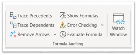
Tracing

The first column of the group allows you to Trace Precedents and Dependents. Precedents are the cells that are referenced in the formula of the currently selected cell. Dependents are the cells that use the result of the currently selected cell in a formula elsewhere on the spreadsheet.

If the link is on the same worksheet, then blue arrows are used to show where the reference lies. If the link is on another worksheet, then a dashed black line connects to an icon. Clicking on the line or icon reveals the Go To dialog box listing all the cell references where the current cell reference is linked.

If you have clicked the link and jumped to another worksheet, you can use F5 Enter to return to the cell where you started.

The third function in the first column is to remove any arrows that have been displayed.

The benefit of this function is to help you discover cell connections and find where values are being applied. Some examples:

• Perhaps three inflation rates are being used in a model (payroll, selling prices and RPI). You might want to identify where each one has been used to ensure the correct rate has been selected.
• You may have discovered an assumption error and therefore need to ascertain where it is been applied in all subsequent calculations.

Error Checking

There are three options available under this item.

Error checking

Excel is constantly checking for errors and will highlight these for you. Under Excel Options (found by selecting the File Ribbon and Options at the bottom of the left column), in the Formulas area you will see Error checking. If you select ‘Enable background error checking’ then Excel will place a small green triangle (or any other colour you choose) in the top left corner of every cell it considers may contain an error. In the block below you can select which errors you would like it to capture.

By using the error checking function in the Formula Auditing Group you can work through all of these errors and Excel will help you resolve them. The following dialog box appears.

It can provide help, use the tracing (described above) to link back to where the source of the error may lie, it can be ignored or edited.

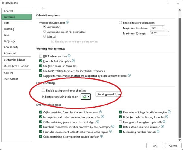
In any spreadsheet review it is worth enabling error checking and working through all the errors this function identifies.

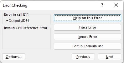
TRACE ERROR

This function will apply Trace Precedents (described above) on the first error it encounters on the current worksheet.

CIRCULAR REFERENCES

A circular reference is created when a formula directly or indirectly refers to itself. The spreadsheet stops calculating when one in encountered and thus spreadsheet values cease to change as data is entered.

The presence of a circular reference is noted in the bottom left corner of the spreadsheet with the cell reference of the first occurrence that it cannot resolve. This function in the Formula Auditing Group will display the cell references of the first two circular references it discovers and by clicking on the cell reference it will jump to where the error resides.

Evaluate formula

This function will calculate each component of a formula step by step. On each click of the ‘Evaluate’ button it will perform one calculation and then simplify the formula to display the answer and remove the function used to derive the value. However, the formula in the selected cell is left untouched, it is only in this function that it is dismantled.

For example, the following formula is used to turn a payback (calculated as a decimal in cell D57) into a text value showing the number of years and months.

By pressing Evaluate the first D57 turns into 2.89353394254 . Another press and it is multiplied by 12 to show 34.7223953. A third press and it is rounded to a whole number to show 35 and so on.

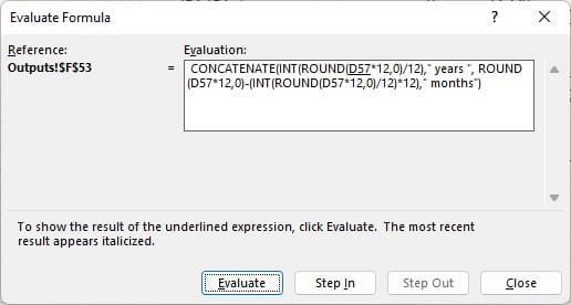
The benefit of this function is that it can be used to slowly unpick a complex formula and check each component. In reviewing a spreadsheet, even if there is no error showing, it may be helpful to simply check the complex formula are correct.

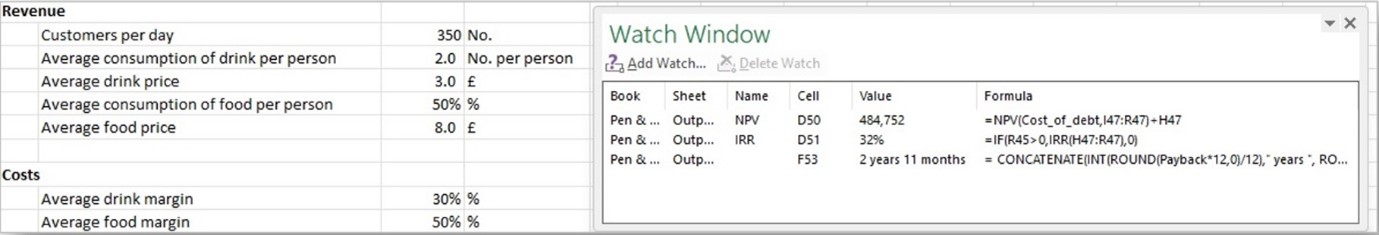
Watch window

The Watch Window allows you to see the results of selected cells as the spreadsheet changes. The window sits on top of the spreadsheet, so it stays present as you move from worksheet to worksheet.

At the top of the watch window are two buttons. One to Add a watch reference and the other to Delete a watch reference.

This a very helpful function for when exploring test data – you can be entering data on an input sheet, yet with this window you can immediately see how a set of output values are changing.

In our final blog 6 we will look at other useful functions and tools including hidden spreadsheet attributes, Inspecting the workbook and more.