Excel Tip of the Week #434 - Revisiting making sets of PivotTables

How to set up your PivotTable

The tool we are examining today is all about filtering your pivot. The idea is to take a pivot that has a filter applied to it, and create a copy of that pivot for each possible option within the filter. This lets you quickly create comparable analyses for each subcategory.

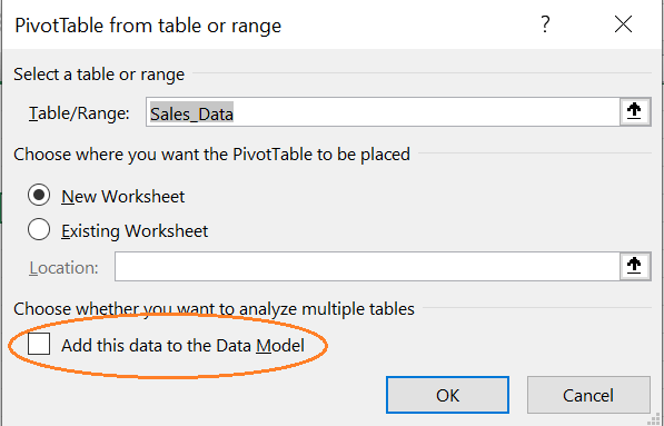
The first thing to note when getting our pivot set up is that this option is not available for pivots based on the data model. Therefore, when inserting your PivotTable, make sure that “Add this data to the Data Model” is unchecked:

You can then build your pivot in the usual way. Any layout or combination of fields is fine – just make sure that you have at least one Report Filter added. Here’s our example using order data, where we have the order dates as row labels and the total order value as the values:

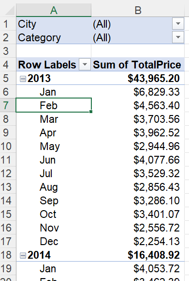
Note that we have for this example included two report filters – the city that the store making the order is in, and the category of the items they have ordered.

Creating the report filter pages

Once you have completed your initial setup, it’s time to hand over to Excel for the automated part.

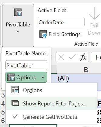
In this example we’re going to create a version of this report for each city. We go to PivotTable Analyze => PivotTable => Options => Show Report Filter Pages:

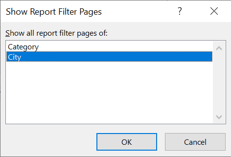
From here we’re prompted to select which of the two current filters we want to cycle through:

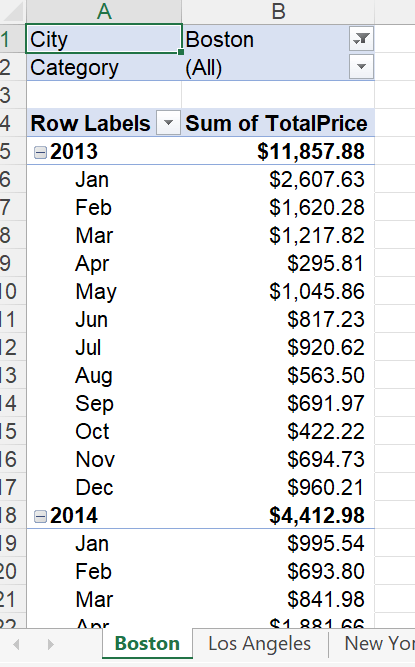
After selecting City, Excel automatically creates new sheets named after each city, each containing a copy of our original pivot but filtered to that city:

Note that there’s nothing keeping these new pivots filtered this way, and nothing tying them to any changes in the layout of the original pivot either – so do be careful that you don’t start making changes to the original and expecting them to cascade through, and don’t make alterations to the filtered versions instead of the original and end up with a confusing workbook.

Incidentally this process is extremely easy to trigger using VBA – for example here’s a recorded macro of the above process:

Sub Report_filter_pages()

    ActiveSheet.PivotTables("PivotTable1").ShowPages PageField:="City"

End Sub

This means that it is possible to automate the creation of these reports. In particular, one thing you might want to do is to create two or more interrelated sets of reports – continuing our example, you might to generate a report for each combination of city and category. There is a macro in the attached file that can do that – just highlight the names of the filters you want to report on at the top of the screen and then run the macro.

• Previous post - Revisiting Excel file types 
• TOTW index 
• Next time – Working with times!