Repeatable calculations with dynamic arrays - part 4: main formula

You can refer to our example Excel file here.

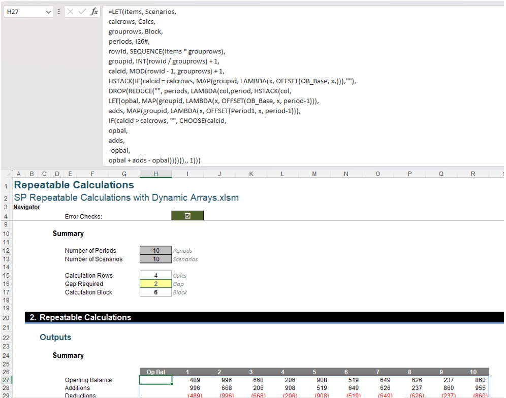
So last week's article covered the easy one! The main block requires a "slightly" more sophisticated formula. You might want to sit down at this point…

=LET(items, Scenarios,

calcrows, Calcs,

grouprows, Block,

periods, I26#,

rowid, SEQUENCE(items * grouprows),

groupid, INT(rowid / grouprows) + 1,

calcid, MOD(rowid - 1, grouprows) + 1,

HSTACK(IF(calcid = calcrows, MAP(groupid, LAMBDA(x, OFFSET(OB_Base, x,))),""),

DROP(REDUCE("", periods, LAMBDA(col, period, HSTACK(col,

LET(opbal, MAP(groupid, LAMBDA(x, OFFSET(OB_Base, x, period-1))),

adds, MAP(groupid, LAMBDA(x, OFFSET(Period1, x, period-1))),

IF(calcid > calcrows, "", CHOOSE(calcid,

opbal,

adds,

-opbal,

opbal + adds - opbal)))))),, 1)))

The first seven rows of this lovely formula are simply defining variables and use the same naming convention as previously, ie, lower case range names have been defined by LET and will therefore only be recognised by LET, and those starting with a capital letter are "traditional" range names, ie, they will be recognised in other Excel formulae.

• items is defined as Scenarios, and has a current value of 10 in our example.
• calcrows is defined as Calcs, and has a current value of four [4] in our example.
• grouprows is defined as Block, and has a current value of six [6] in our example.
• periods is equal to the dynamic array range starting in cell I26 (see image above). This is the horizontal column counter in our example:

• rowid is defined as SEQUENCE(items * grouprows), which generates a column vector of the integer values one [1] through 60.
• groupid is defined as INT(rowid / grouprows) + 1, which generates another column vector. This one essentially identifies a calculation block by generating the numbers
  {1, 1, 1, 1, 1, 2, 2, 2, 2, 2, 2, 3, 3, 3, 3, 3, 3, 4, 4, 4, 4, 4, 4, 5, 5, 5, 5, 5, 5, 6, 6, 6, 6, 6, 6, 7, 7, 7, 7, 7, 7, 8, 8, 8, 8, 8, 8, 9, 9, 9, 9, 9, 9, 9, 10, 10, 10, 10, 10, 10, 11}.
  The formula could be refined to make each cycle of six [6] the same value, but it is not necessary as there is always a blank row at the end (see later). It only matters the calculation rows show the correct calculation number.
• calcid is defined as MOD(rowid - 1, grouprows) + 1, which generates the column vector
  {1, 2, 3, 4, 5, 6, 1, 2, 3, 4, 5, 6, 1, 2, 3, 4, 5, 6, 1, 2, 3, 4, 5, 6, 1, 2, 3, 4, 5, 6, 1, 2, 3, 4, 5, 6, 1, 2, 3, 4, 5, 6, 1, 2, 3, 4, 5, 6, 1, 2, 3, 4, 5, 6, 1, 2, 3, 4, 5, 6}
  as before.

Immediately after the definition of the calcid variable, we have the expression

HSTACK(IF(calcid = calcrows, MAP(groupid, LAMBDA(x, OFFSET(OB_Base, x,))),""), Horror_Formula)

Let's leave the Horror_Formula aside and concentrate on the first part. HSTACK effectively combines columns and the formula

IF(calcid = calcrows, MAP(groupid, LAMBDA(x, OFFSET(OB_Base, x,))),"")

defines the first column. As explained above, calcid in this example is cycling through the integers one [1] through six [6] a total of 10 times. This will generate a column of 60 rows. Using the MAP LAMBDA trick explained earlier, whenever the value of calcid equals the calcrows (Calcs) value of four [4], it will effectively take the corresponding result of

OFFSET(OB_Base, groupid,)

Similar to Labels earlier, OB_Base has been defined as the cell containing "Op Bal" in the inputs table, viz.

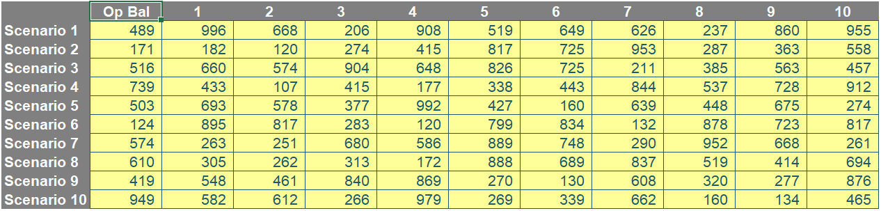
Therefore:

• the first computation will occur in the fourth row of the column vector, where the corresponding groupid value will be one [1] and the value returned will be the Opening Balance for Scenario 1 (489 in our image).
• the second computation will occur in the 10th row of the column vector, where the corresponding groupid value will be two [2] and the value returned will be the Opening Balance for Scenario 2 (171 in our image).
• etc.

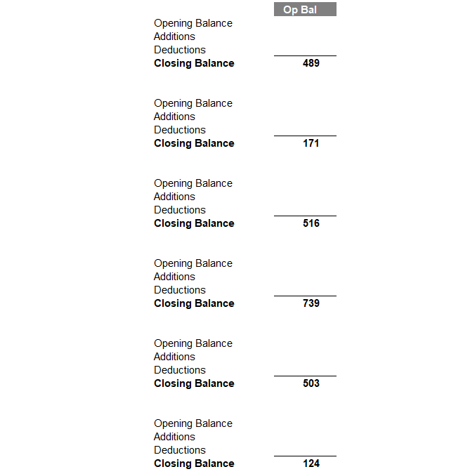
Put simply, whenever the row represents the position of the final calculation in the block, the Opening Balance will be displayed, otherwise the cell will be empty (“”).

The HSTACK formula merely combines this with the computations for all of the periods, which is the Horror_Formula cited above.

The next part of the formula (viewing right through to the end) is

DROP(Long_Calculation,,1)

This assumes Long_Calculation produces an array and it will remove the first column of the array produced. That's not too hard to follow. Therefore, it begs the question, what is the array produced?

REDUCE("", periods, LAMBDA(col, period, HSTACK(col, More_Calcs…

Ignoring the More_Calcs aspect of the above formula, REDUCE will reduce the rest of the calculations to an "accumulated value", which here will in effect be an array of 60 rows by 11 columns – not 10 when More_Calcs is taken into consideration. This is because there is an initial value (“”) – hence the need to remove this first "starter" column with the DROP function above.

REDUCE uses the starter value of “” (which no doubt will cause errors in the later formulae, but it doesn’t matter as it will be removed). It should be noted that we cannot leave this starter value argument empty even though it is optional. This is because HSTACK will not work with empty ranges / arrays and therefore will return an #VALUE! error.

This formula then continues for periods (here, 10) more times, where a LAMBDA will define the starter value of the empty range / accumulator (col) and then consider each period separately. Read the formula carefully: the value periods is the array of integer values one [1] through 10, whereas period considers each value separately in the following calculations. There is no typographical error in the formula. More_Calcs is going to return a column vector each time (one [1] column by 60 rows) and HSTACK will simply combine them.

It is all of above in this Main Formula section that you will replicate for other blocks of repeatable formulae. What follows now is specific to the calculations created here. You may need to use alternative MAP LAMBDA combinations to create your formulae, but the idea remains the same.

What now remains is

LET(opbal, MAP(groupid, LAMBDA(x, OFFSET(OB_Base, x, period-1))),

adds, MAP(groupid, LAMBDA(x, OFFSET(Period1, x, period-1))),

IF(calcid > calcrows, "", CHOOSE(calcid,

opbal,

adds,

-opbal,

opbal + adds - opbal)))

We start with more definitions of required calculations:

• opbal simply cycles through groupid
  {1, 1, 1, 1, 1, 2, 2, 2, 2, 2, 2, 3, 3, 3, 3, 3, 3, 4, 4, 4, 4, 4, 4, 5, 5, 5, 5, 5, 5, 6, 6, 6, 6, 6, 6, 7, 7, 7, 7, 7, 7, 8, 8, 8, 8, 8, 8, 9, 9, 9, 9, 9, 9, 9, 10, 10, 10, 10, 10, 10, 11}
  and then uses the OFFSET function OFFSET(OB_Base, groupid, period-1) to return the correct value. Due to how the Control Account is defined, this is simply the values in the input table for the given scenario.  We have to use period-1 as the number of columns to move to the right (rather than period) as DROP will remove the first column, and we need to move no columns for the first period [1], one column for the second period [2], and so on.
• adds works similarly, but has a different starting point, using OFFSET(Period1, groupid, period-1). Period1 is simply the heading cell for the first period, viz.

• Arguably, we could have used OB_Base again and changed the column movement to period instead.

We do not need to define the Deductions and Closing Balance as the deductions are simply the removal of the opening balance, and the Closing Balance is simply the aggregation of the other elements.

The calculations-specific formulae are now built. The first part,

IF(calcid > calcrows, "",

ensures that blank rows are entered in the cycle once the number of calculations required (Calcs, which is four [4]) have been performed for the Block. This restricts how many elements we need in our final expression, the CHOOSE formula:

CHOOSE(calcid, opbal, adds, -opbal, opbal + adds - opbal)

You may need more than four choices in your set of calculations. It depends on the Calcs figure. Here, if calcid

{1, 2, 3, 4, 5, 6, 1, 2, 3, 4, 5, 6, 1, 2, 3, 4, 5, 6, 1, 2, 3, 4, 5, 6, 1, 2, 3, 4, 5, 6,
1, 2, 3, 4, 5, 6, 1, 2, 3, 4, 5, 6, 1, 2, 3, 4, 5, 6, 1, 2, 3, 4, 5, 6, 1, 2, 3, 4, 5, 6}

is:

1. It will display opbal
2. It will display adds
3. It will display the negative value of opbal
4. It will sum the above, which is opbal + adds – opbal (yes, I know I could have just written adds, but it has been expressed this way for "clarity").

And that's it: you now have your resulting array when it is all combined, viz.

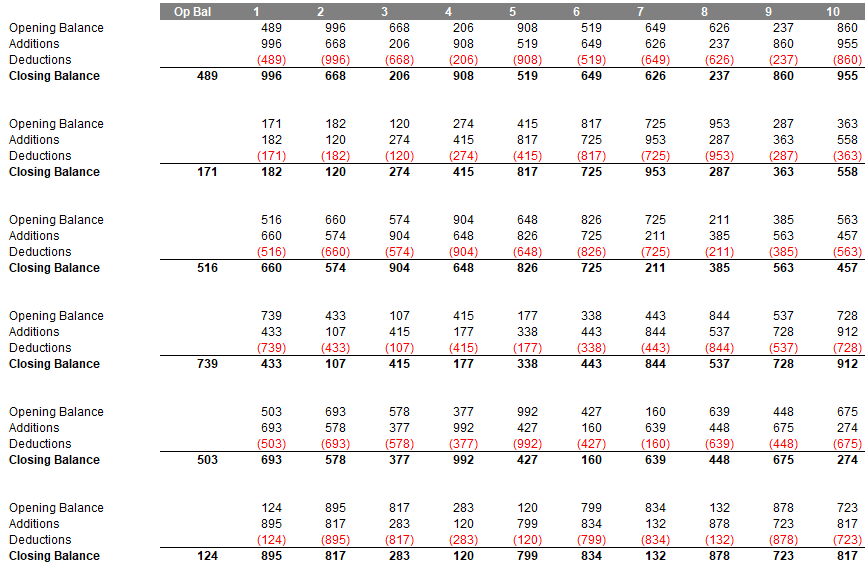
You will need to add conditional formatting for borders and emboldening, but this can be checked out in the attached Excel file.

Word to the Wise

It's true this all looks pretty horrible, but much of the formula is "repeatable" (pun intended). If you use the same range names I have employed, effectively all you need to do is create the formulae for the calculation block (ie, write your equivalent opbal, adds, etc. calculations). It is simply a calculation engine.

One other advanced point to note if you plan to use closing balances. In array (and for that matter, DAX) formulae, closing balances usually need to be aggregation formulae (ie, summing all movements to that point). This is avoided here due to specifically using this Control Account. This was in order to highlight the approach and not include unnecessary complications.

And if you are feeling even "more advanced", perhaps you can modify the formula to turn it into its own LAMBDA and simplify the formula!! 

Further resources

• Repeatable calculations with dynamic arrays - example Excel file
• Repeatable calculations with dynamic arrays - part 1: introducing the technique
• Repeatable calculations with dynamic arrays - part 2: key functions
• Repeatable calculations with dynamic arrays - part 3: labels calculations