
Legacy Excel supports a range of functions and techniques that can help identify potential errors and problems within a spreadsheet as part of a review process. In part 1 of this series, we looked at some of the advantages of adding Power Query to your review toolkit. This time we are going to move on from the Profile table that we created in Part 2 to rearranging our Table and positioning it above our original data for ease of reference. We will be using a range of techniques that demonstrate the versatility of the Power Query tools.
Errors in data
We started the series by using Power Query to quickly reveal some key information about the contents of columns in a table of data. We moved on from the display of this information to seeing how the Power Query Table.Profile function could be used to create a more permanent report. This time, we are going to arrange this table above our original table of data in order to combine the raw data, and the summary profile, on the same page.
Prepare to Transpose
Reorganising our table in this way adds a few complications but, to start with, we just need to make room to fit our Profiles table above our Invoices table in our worksheet, so we will insert 10 rows above our table and insert one column to the left.
Transpose
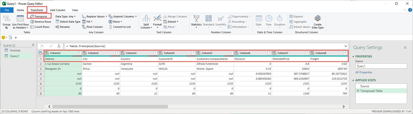
We now need to reorganise our Profiles query output. First of all, because our Profiles table shows the information related to each original data column by rows, we need to swap our Profiles table round so that our column information is shown in columns rather than rows. Although we can transpose a table with the simple Transpose command in the Table group of the Transform Ribbon tab, this moves our column names into the data area and rearranges them in alphabetical order:
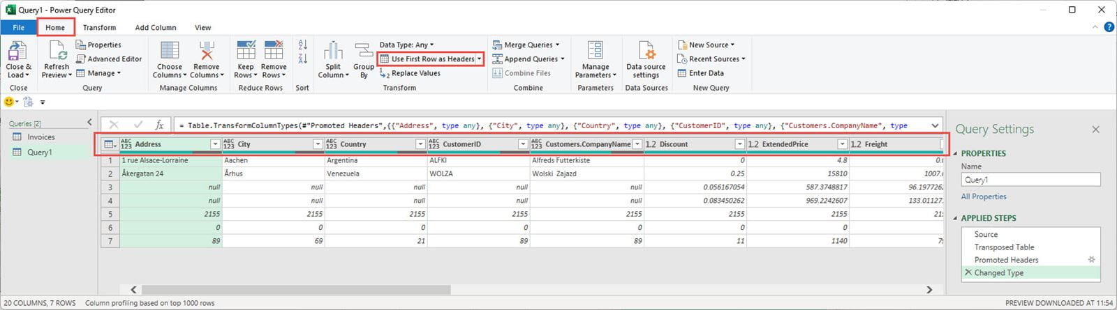
Restoring the column names as headers is straightforward. From the Home Ribbon tab, Transform group we can just click on the Use First Row as Headers command:
There are other issues. The Transpose command has removed the column headers which contained the descriptions of our profile rows. To prevent this, we use the ability of Power Query to allow us to travel backwards in time. We click on our first, Source, step which still has our descriptions as column headers. Then we the ‘Use Headers as First Row’ dropdown and choose ‘Use First Row as Headers’ to include our descriptions as the first data row of our table. After a warning about inserting a step, our descriptions will appear within the data area so that when our table is transposed by the subsequent step, they will be included as the leftmost column. We don’t need to change any of our existing steps and can just click on the last step in our query to confirm that we have our additional Column containing our profile descriptions.
Unfortunately, our columns remain in alphabetical order. There are probably several ways to deal with this, including manually rearranging the columns, but we will use a quicker, if somewhat less obvious, method.
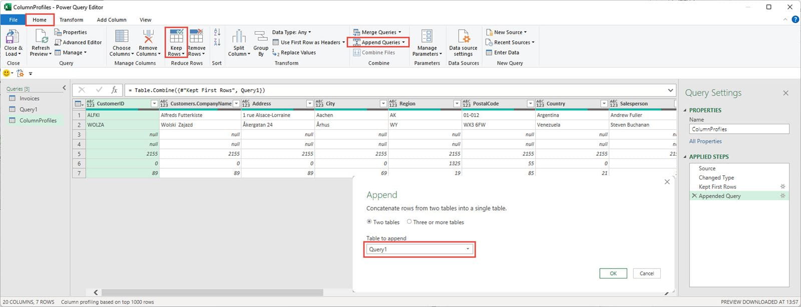
First, we right-click on our Invoices query and use the Reference command to create a new query that uses the existing Invoices query as its data source. This ensures that any change in our Invoices query will flow through to our new query, which we have renamed ‘ColumnProfiles’. Next, we take the rather unusual step of deleting all the rows of our new query by using Home Ribbon tab, Reduce Rows group, Keep Rows, Keep Top Rows and setting the number of rows to 0. All we have left is a query that just contains our column headers. We use Home Ribbon tab, Combine group, Append Queries and choose to add our Profiles query to our empty query. This has the effect of leaving the data exactly as it is, but rearranging the columns back into the original order, with the addition of our profile descriptions column:
For clarity, we might want to move the additional column containing the profile descriptions to become the leftmost column by right-clicking on the column heading and choosing Move, To Beginning. We can then use the Close and Load dropdown, Close & Load To… command to load our query to cell A1 of the sheet containing our Invoices table:
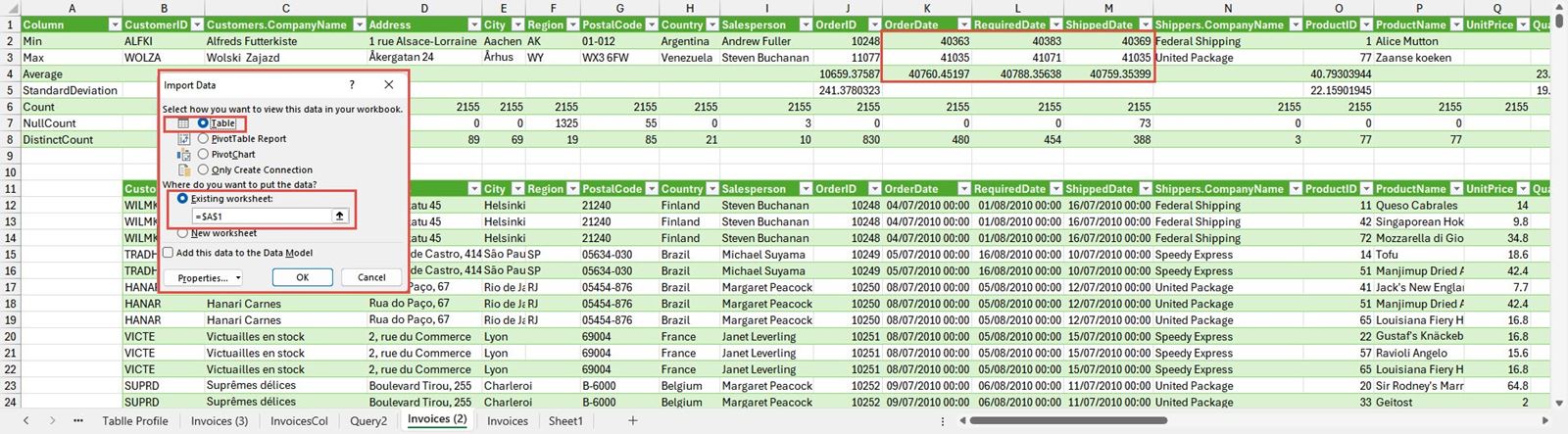
Note that it is not generally a good idea to combine output tables on the same sheet, as overlaps can prevent Tables refreshing properly. However, in this case, our top table includes more columns and extends at least as far across the worksheet columns as the table beneath, so it will move the entire lower table down if the number of rows increases.
Formatting
The columns containing dates create another issue. Some of the profile information, such as the various counts, are integers, whereas the Minimum, Maximum and Average values can be dates. Power Query treats them all as numbers, so we would need to separately format the cells containing dates in the date columns in the output table so as to display them as dates rather than numbers.
Conclusion
Having created our profiles table and seen how we can combine it with our underlying data table, in part 4 we will go on to see how our profile table deals with Power Query errors and examine some further checks that we could build in.
You can explore many of the various techniques we have covered here, and a great deal more, in the ICAEW archive:
Archive and Knowledge Base
This archive of Excel Community content from the ION platform will allow you to read the content of the articles but the functionality on the pages is limited. The ION search box, tags and navigation buttons on the archived pages will not work. Pages will load more slowly than a live website. You may be able to follow links to other articles but if this does not work, please return to the archive search. You can also search our Knowledge Base for access to all articles, new and archived, organised by topic.
