How to review a spreadsheet: Part 4 - design principles and formula errors

Design principles

As mentioned in part 1, the primary way to avoid error in a spreadsheet is to build the spreadsheet correctly at the outset. We will look in this section at some functions that allow us to inspect the spreadsheet to ensure appropriate construction.

Hard Coded Numbers – All data should be stored on a sheet of inputs and referenced when included in formulas. A piece of data keyed directly into a formula, or a balancing figure used to remove rounding can corrupt functionality especially when alternative scenarios are being explored. To discover any hard coded numbers there are two useful functions.

On the Formulas Ribbon in the Formula Auditing section is the Show Formulas option (also available by CTRL `). This will turn your spreadsheet from displaying results to formulas. It is much easier to scan cells for consistency and hard coded numbers in this mode than inspecting them one by one by placing the cursor on each cell to see its formula.

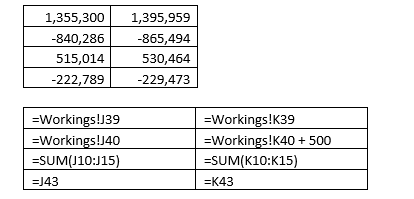
For example, the block of cells below, when switched to formula view reveals a hard coded + 500.

Another option is Go To Special that can be used to highlight a variety of criteria. Press the F5 button at the top of the keyboard and the Go To function is revealed (useful for jumping to the locations of Range Names). In the bottom left of this dialog box is the Special… button.

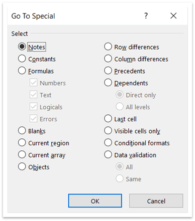
The following dialog box of options is displayed.  Select the criteria required such as Constants (typed in numbers) and on pressing OK all incidents in the workbook of that criteria are highlighted in mid grey. These can now be individually validated.  However, as soon as any cell is selected the grey will disappear.

Please note that selecting constants will only pick out cells comprising solely of numbers, it does not pick out cells where numbers have been added to a formula (as illustrated above).

Unused Inputs – An input that has not been refenced in the spreadsheet is not necessarily an error, but it does the beg the question ‘why is it there?’. To find these values you can use the Trace Dependents function on the Formulas Ribbon in the Formula Auditing section. By applying the function to a cell a set of blue arrows will appear where it used on the same sheet or a Go To dialog box link to where it used on other worksheets. If no links are found an error message is displayed. To remove the arrows there is a button in the Formula Auditing section to do so.

External Links – Where source data is drawn into the spreadsheet by a link to another spreadsheet it is easy for incorrect data to be used. This is either through a lack of refreshing the link so old data is being used or because the source sheet has had formula revision such that it no longer passes the correct information across.

To update links and ensure the latest information is being used go to the Data Ribbon and in the Queries & Connections section click on Edit links. If this button is greyed out it means that there are no Links used in the spreadsheet.

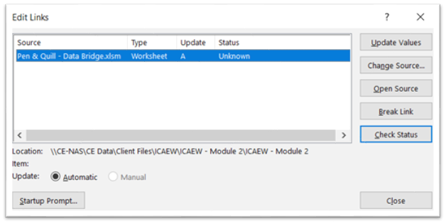
The values can now be updated and in the bottom left corner the updates can be automated at start up.

Any spreadsheet review should of course include a review of any Linked sheets. This dialog box is a helpful way to identify if any links exist and determine the scope of any further review.

Formula errors

We will pick up some types of formula errors in later blogs such as circular references and hidden calculations. We look here at some of the potential errors that functions can create.

Indirect Addresses – Functions such as =OFFSET and =INDIRECT create cell address references by using cell values. Consequently, it can be difficult to verify that they are referring to the correct cell.  For example a small currency selection option below uses =OFFSET to determine the rate to use from the table.

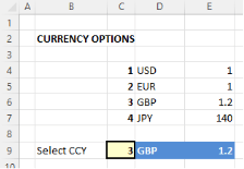
The formula in cell E9 is =OFFSET(E3,C9,0)

If the user were to enter in C9 a value of 5, for which no currency exists, but is a blank cell on the worksheet this will result in a null result.  But if the user entered a much higher number this might align to a value further down the spreadsheet that would give rise to an error.

To hunt for the use of these functions (sometimes referred to as volatile functions due to the uncertainty of validating their result) use the Find function on the Home Ribbon in the Editing Group (CTRL F).  The review needs to check how the result is controlled and the implication of an errored link.  In the example above the entry in Cell C3 could be checked by either Data Validation – see blog 2 or a Test in F9 that validates the number entered is in the correct range or displays an error message.

Nested =IF and =IFS – An =IF statement performs a logical test (true or false) and returns one of two outcomes.  Nesting is where another =IF test us used within the outcome field of a previous =IF test.  If there are multiple =IF tests all nested inside of each other (Excel will allow up to 64) then this becomes very difficult to manage let alone review.  Where these occur, the nesting should be broken down across several rows rather than built all in one cell.  It may also be possible to change the structure of the nesting to a table. With the correct result being found by using =XLOOKUP.

To identify an incident of =IF is easily done by searching as explained above for Indirect Addresses. However, there is no easy way to find multiple incidents of =IF nested within each other.

=IFERROR – This function is helpful in capturing an error and giving a pre-determined result. For example, if a division by zero should occur.

=IFERROR(100/B3,0)  If B3 were zero a #DIV/0! Error would occur, but by placing the calculation within an =IFERROR statement and setting the Value If Error field to zero then no error will be displayed, and the cell will show 0.

However, if B3 had become typed over with letters it would not show as a problem.  Good practice for when =IFERROR is used would be to script the trapping it is designed to handle beside its use.  Thus, in a review the =IFERROR can be removed, and its purpose can be tested and validated by tracing the source and entering zero.

In blog 5 we will look further at the details in the spreadsheet and look at the Formula Auditing group to review some of the error checking functions.