Risk Bubble Charts – Part 2

Bubble Chart

In our first article, we laid the groundwork for our Risk Bubble chart by creating a colour-coded risk table. Now the time has come to add the bubbles to it.

As we mentioned before, we will need to transform the data in the Risk_ Category table to make the Risk Bubble chart. Let’s remind ourselves of the aforementioned table:

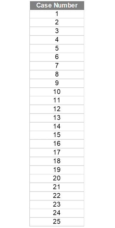
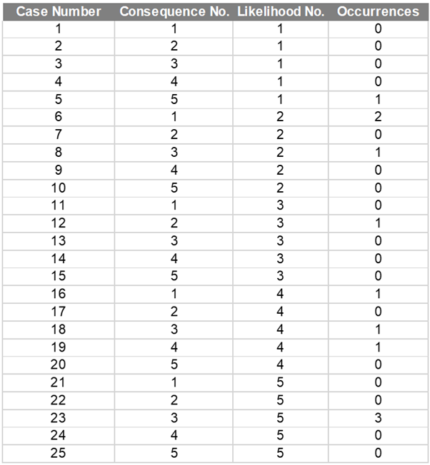
There are five [5] different Likelihood scenarios and five [5] different Consequences scenarios, so there is 25 unique way you can pair the Likelihood scenario with the Consequences scenario (a simple multiplication of 5 x 5). we will create a columnar table that has case numbers from one [1] to 25 and we name the column ‘Case Number’ and we shall name this table Chart_Data:

The next column we will create is ‘Consequence No’ which generate case number from one [1] to five [5] here repeatedly. Why we choose the ‘Consequence No’ column here because when this column feed into chart data it will be the x position of the bubble as we positioned it on the risk table. Anyway, the data for the ‘Consequence No.’ column will look like this:

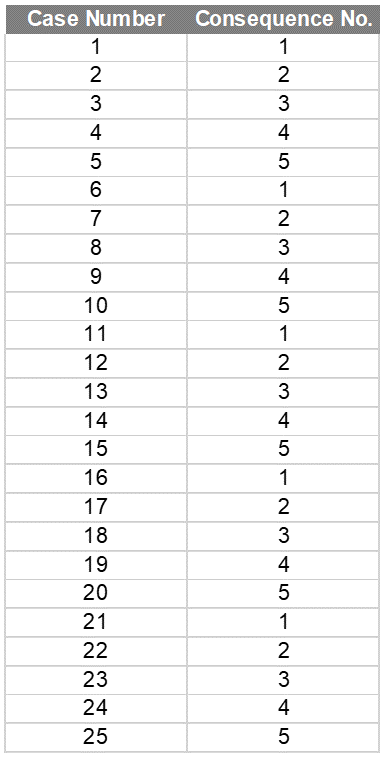
The question now is how we did that. We just need a bit of help with some mathematics here where we take the remainder of a division of the ‘Case Number’ by the number of consequences and if the remainder is zero [0], we will set it as the number of consequences we have. Hence, we can employ the MOD function here (with COUNTA) to do that:

=MOD([@[Case Number]]-1,COUNTA(LU_Consequences))+1

MOD will create a loop of the numbers 0, 1, 2, 3 and 4; subtracting one inside the function and adding it back outside the calculation has the effect of looping 1, 2, 3, 4 and 5 instead.

The next column we will create here is the ‘Likelihood No.’ column. This column will be slightly different from the ‘Consequence No.’ column. In the first row of the ‘Likelihood No.’ column, we will enter the following formula:

=ROUNDUP([@[Case Number]]/COUNTA(LU_Consequences),0)

This formula will give us the following visual:

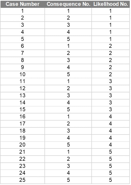
If you have a keen eye, you might spot the problem with the formula above. Why are we using the LU_Consequences here? Well, if you only have three [3] likelihood scenarios here our table can just stop at case number 15 and at that point, it includes all our combinations between likelihood and consequence. If we fixed this formula to employ the COUNTA of LU_Likelihood the combination will not be correct. It seems counterintuitive but it is true.

The next item on the list is the size of the bubble. To determine the size of the bubble, we simply count the occurrence of Risk_Catergory according to their Likelihood and Consequences. Therefore, we will use the following formula:

=COUNTIFS(Risk_Category[[Likelihood]], [@[Likelihood No.]], Risk_Category[Consequence], [@[Consequence No.]])

What this formula generally does is count how many times a specific risk has the same likelihood number and the same consequences number. This creates an Occurrences column as follows:

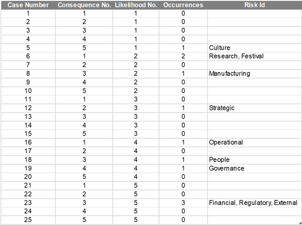
The last column we will have today is ‘Risk Id’. This column function is used to name our bubble, so we will employ the TEXTJOIN function here to help us do that:

=TEXTJOIN(", ", , IF(Risk_Category[Likelihood]=[@[Likelihood No.]], IF(Risk_Category[Consequence]=[@[Consequence No.]], Risk_Category[Risk Category], ""), ""))

This formula essentially looks for the Risk_Catergory that have the same Likelihood and same Consequences and joins them together with the comma as the delimiter between them. This formula will return us the following formula:

At this point we can finally plot our bubble chart. Yay!

We simply select the ‘Consequence No.’, ‘Likelihood No.’ and the ‘Occurrences’ columns without the headers. Then we go to Insert -> Charts -> Bubble -> 3-D Bubble:

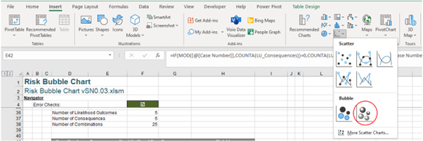
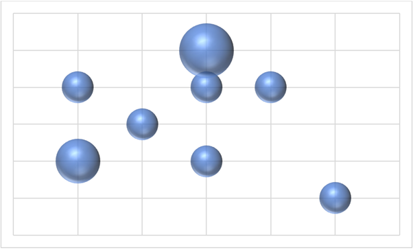
This will give us our Bubble chart:

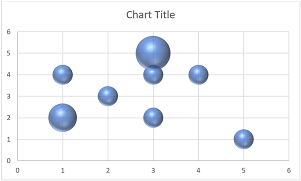
Let’s remove few elements of the chart that we don’t need here:

We then set the ‘Chart Area’ to ‘No Fill’, which will make our chart appear transparent. Then, we place this chart on top of the risk table we created earlier:

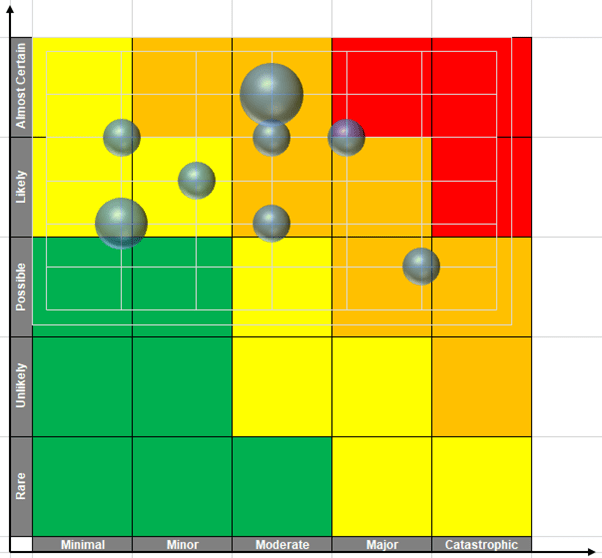
Care is now required to resize the chart so that it will fit the risk table precisely:

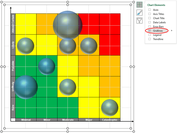
We then remove the Gridlines (either View -> Gridlines or the keyboard shortcut ALT + W + VG) from the chart:

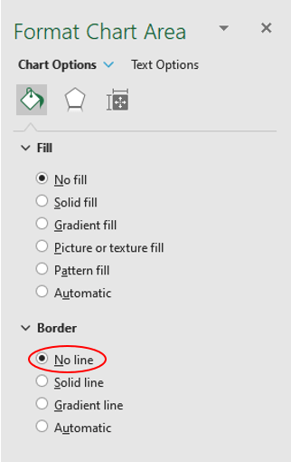
and the border as well:

With this all completed, we may then double-click on the bubble(s). This will give us the following box:

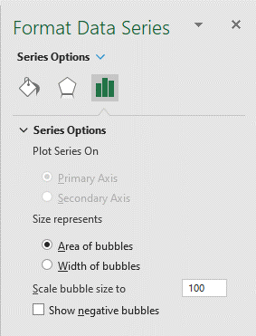
In the ‘Scale bubble size to’ we can set equal to 75, which will provide a nice visual here:

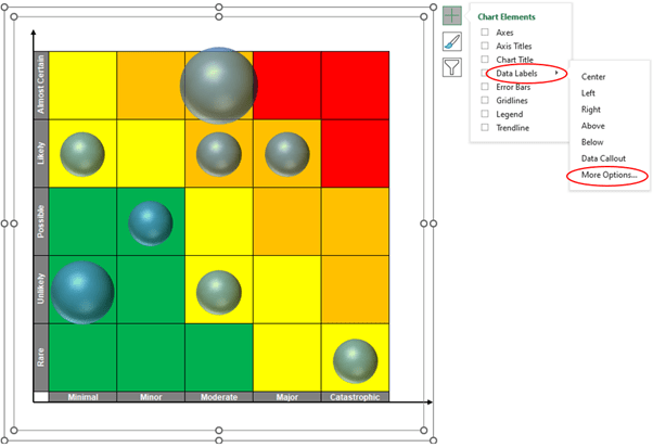
The last step here will be to name the bubbles. We click on the chart and press the plus button on the ‘Data Labels’ row select the black triangle and select the ‘More Options…’:

This will trigger the following ‘Format Data Labels’ pane, where we may select the ‘Label Options’:

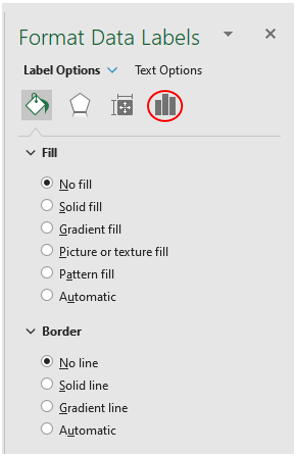
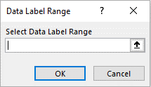
We will untick all the ‘Label Contains’ option that are available here and tick the ‘Value From Cells’. A ‘Data Label Range’ box appears here:

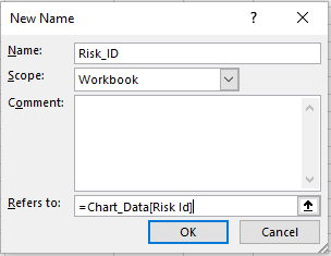
Before we put the data range here, we will name the data in ‘Risk Id’ column as Risk_ID. Why we are doing this is so that this heading will update automatically. For example, we may have more scenarios for likelihood or consequences in the future. Our new name range in the ‘New Name’ dialog will thus look like this:

Returning to the ‘Data Label Range’, we put ‘Risk_ID’ in the dialog as so:

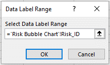
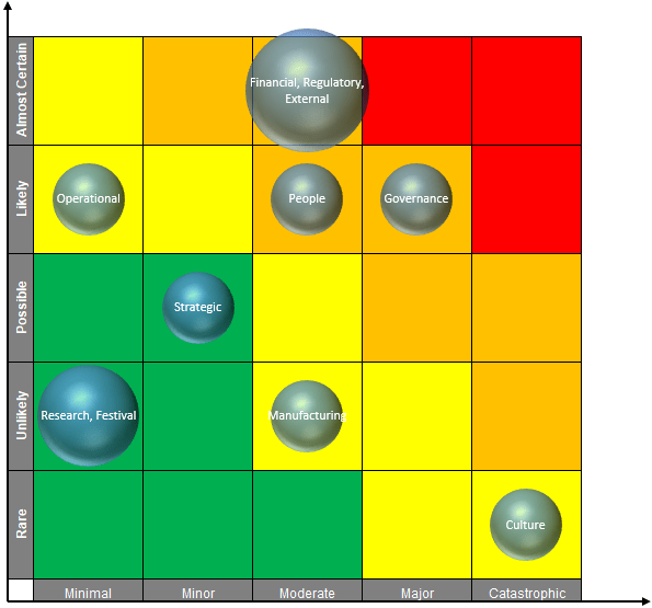
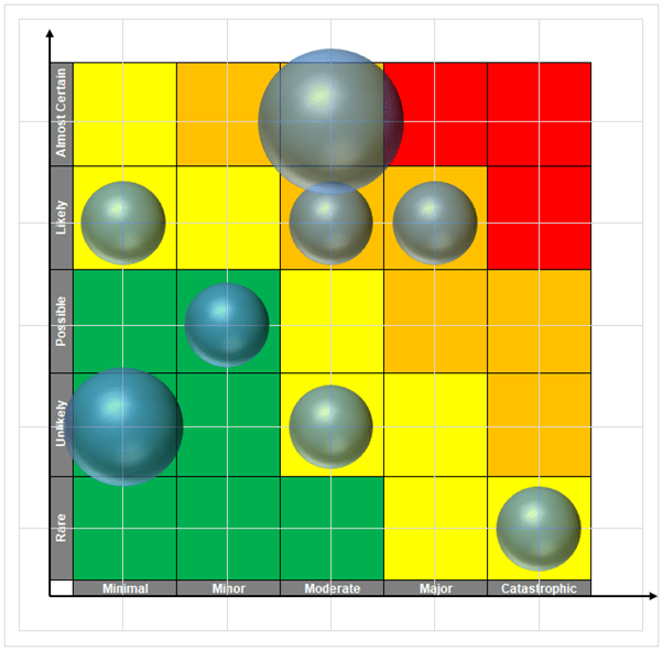
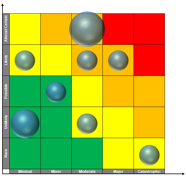
This will ensure that the name of the bubble will be updated together with our table. Our final product will look like this:

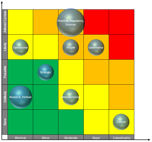
And there we have it – a fully functional, dynamically updating Risk Bubble chart. Take a look at the attached Excel file to see it in action!