
Applying default conditional formats is very straightforward and can be accomplished with just a couple of clicks, but delving a little deeper can help you to use conditional formatting in additional ways and to tailor your format to your own requirements. In the first part of a short series, we look beyond the default formats and include a practical example using number formatting.
Introduction
The conditional formatting feature in Excel can be used very simply, with just a few clicks required to highlight significant cells or to apply one of three types of graphical format to a range of cells. However, taking the time to explore the capabilities of conditional formatting in a bit more detail can help you to extend what you can achieve and ensure that your formatting looks exactly how you want it to.
In the first part of a short series, we will be looking at some of the less obvious options available within the Highlight Cells and Top/Bottom rules sections.
Looking beyond the defaults
When you select a range of values and use the Home Ribbon tab, Styles group, Conditional Formatting dropdown to choose one of the basic Highlight Cells or Top/Bottom rules, Excel will suggest the values and the formatting to be used. This means that you can apply a conditional format with a single click. The values can be changed easily, either to use different values or to refer to the contents of cells. Referring to cells, rather than just typing in numbers, makes it much easier to change the values if required, or to use your own formula to calculate the values.
Here, we have entered a threshold value into cell B1 and then set up a Highlight Cells, Greater Than… rule where we have set the trigger value to refer to B1 so that a user can change which values are highlighted, simply by changing the value in the cell:
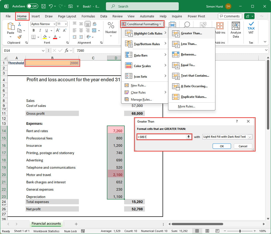
With regard to the formatting, a dropdown allows you to choose from six basic formats based on text colour, cell fill colour and a coloured border. There is also a Custom Format option that opens a simplified Format Cells dialog so that you can choose whichever format attributes you want:
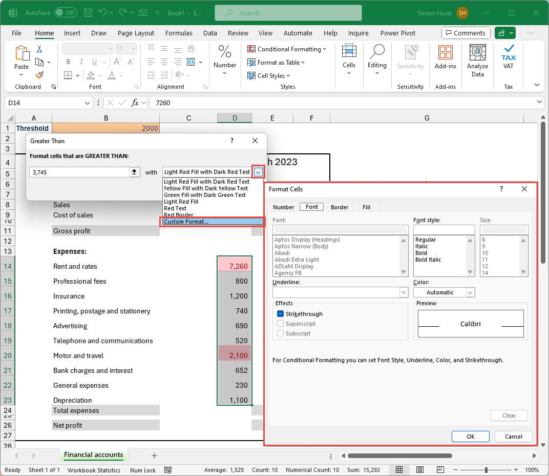
As well as giving you the full range of text colour, cell fill colour and border options, there are several additional formatting options available. Some text attributes apart from colour can be used as part of the conditional format: strikethrough; font style (bold and italic); single or double underline. For Cell Border, the style and colour of each of the four cell borders can be chosen individually. For Cell Fill, as well as choosing any colour, it is also possible to use gradients and patterns. In addition, conditional formatting can use the options in the Number tab of the Format Cells dialog. So, for example, you could change the currency symbol displayed for values depending on the value in a particular cell. Note that neither the Alignment nor Protection tabs from the full Format Cells dialog are available as part of conditional formatting.
As well as being able to go beyond the defaults for the specific rules in the Conditional Formatting dropdown, it is also possible to use the More Rules… option at the bottom of each dropdown list to use a formula instead of any of the built-in rules. The formula can use Excel functions and needs to return a TRUE or a FALSE value. When the return value is TRUE, the formula will trigger the conditional format.
In this example, we are combining the use of a formula-based rule with the use of the Number section of the Format Cells dialog to allow the user to set the currency symbol used as part of the number format based on the contents of a specific cell. We have formatted a set of numbers to use the £ symbol and allocated the Range Name ‘Currency’ to cell B2. This cell uses Data Validation to allow the user to select Dollar or Sterling from a list.
Our formula is:
=(Currency=”Dollar”)
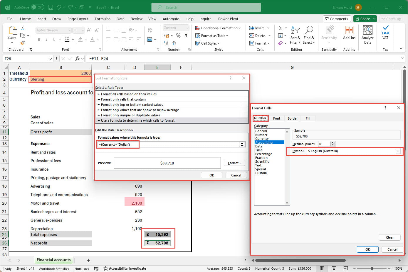
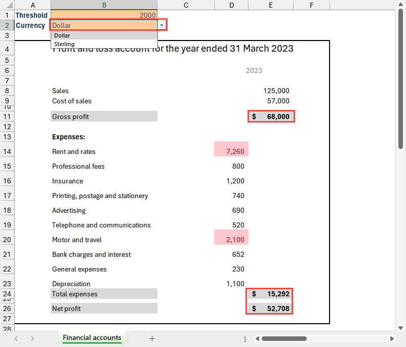
When the user chooses Dollar from the Data Validation dropdown, the conditional format changes the Number format to use the $ symbol instead of the £ symbol:
Any colour you like
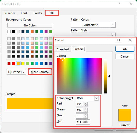
Throughout all the conditional formatting options the choice of colour goes beyond the normal selection of Standard and Theme colours. The More Colours… option allows you to select very specific colours, including using RGB values to match a particular brand colour scheme if necessary:
Conclusion
Next time, we will begin exploring the graphical conditional formats and see how to work with the less obvious options, such as the colour of negative bars and the addition of highlight blobs.
For more articles on conditional formatting, search the ICAEW Excel Community article archive:
Archive and Knowledge Base
This archive of Excel Community content from the ION platform will allow you to read the content of the articles but the functionality on the pages is limited. The ION search box, tags and navigation buttons on the archived pages will not work. Pages will load more slowly than a live website. You may be able to follow links to other articles but if this does not work, please return to the archive search. You can also search our Knowledge Base for access to all articles, new and archived, organised by topic.