Excel Tips & Tricks #474 - How to REDUCE repetitive calculations to a single step

REDUCE is a relatively new function, having been introduced in 2021, and is available to users of Office 365. The basic idea is that it takes an initial value, then performs a calculation for each value in a target array then returns the output as a single value.

Why is that useful, you may ask? Well, broadly speaking REDUCE can be useful in the following scenarios:

1. Aggregating numeric values that meet certain criteria.
2. Cleaning up text data by removing unwanted characters.

The logic that underpins that accumulation is provided as a LAMBDA function. Don’t worry if you’ve never seen or heard of LAMBDA functions before! For this article we are not assuming any prior knowledge of LAMBDA functions, just a basic familiarity with building formulas in Excel – though if you do want to learn more, we covered LAMBDA functions in Tip #459.

The main concept here to understand is the chain of calculations that underpins the calculation. We will build the intuition first by way of examples before digging into the syntax of the REDUCE and LAMBDA functions.

Example 1 – adding a list of numbers

In the first example we are simply taking our initial value and adding on all the values in the target array, one by one, until we get our final output.

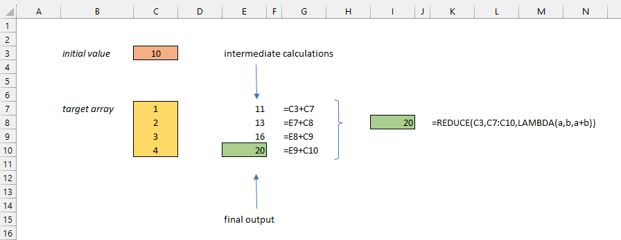
On the right-hand side, we are showing how the same result can be achieved in a single REDUCE function.

This is obviously a trivial example; in real life applications you would simply use the SUM function for this task. But by following the step-by-step logic at this stage we set the scene for more advanced applications of the REDUCE function.

Example 2 – adding numbers using custom criteria

In the second example we are looking to add all the even numbers in our target array (by using a combination of the IF and ISEVEN functions). This is not something that can be achieved with standard applications of the SUM or SUMIF functions.

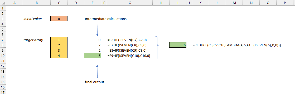
As you can see the final output is the sum of the even numbers in the list: 2 + 4 = 6.

Here we are starting to tap into the power of the REDUCE function by using it in combination with the IF function.

Example 3 – text clean-up operations

The final example (before we dig into the syntax of the REDUCE function) considers text instead of numbers. Here we are looking to clean (i.e., remove) the characters in the target array from the initial value by repeated application of the SUBSTITUTE function:

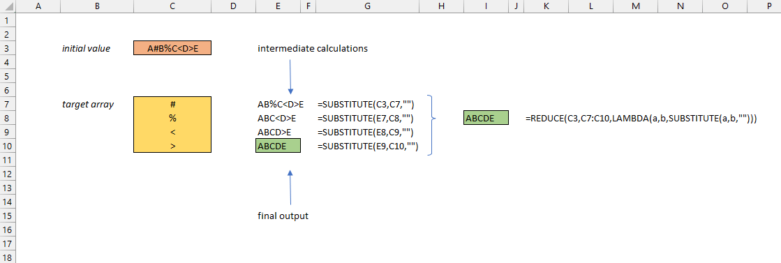
Here we have an initial value containing characters that we don’t want (#%<>). The REDUCE function removes each of these in turn leaving the desired output without just the clean text.

REDUCE function in detail

Here we take a closer look at the syntax of the REDUCE function:

= REDUCE ( initial value , target array , LAMBDA function )

Taking each argument in turn:

initial value
The initial value is exactly that. This is the starting point for your calculations.

target array
The target array is the range of cells containing the values that will be passed one by one into our calculation.

LAMBDA function
This is where the magic happens! The syntax for the LAMBDA function is as follows:

= LAMBDA ( first parameter , second parameter , calculation )

• The first parameter will keep track of the calculated value that is passed from one calculation to the next (see the intermediate values in column E in the examples above). We can choose any name we want for this parameter, so let’s keep things simple and choose the letter “a”.
• The second parameter allows you to refer to each value of your target array in turn. Again, we can choose any name, but for simplicity let’s choose the letter “b”.
• Finally, we build the calculation with any valid Excel formula. We can refer to the first and second parameters above, using the names we have chosen, “a” and “b”. The calculation will be performed for each value in the target array, building one long chain of calculations from the initial value to the final output of the reduce function.

Why REDUCE?

In summary the REDUCE function can help you to reduce a set of values into a single value. By using the power of LAMBDA, you can simplify tasks that may previously have taken many repetitive calculations to complete.