Excel Tips & Tricks #473 – Refreshing customising the ribbon

This was last covered back in Tip #312.

The Ribbon replaced dropdown menus in Excel 2007, and since then has been a fixture of the Office suite. The default set of menus can be added to - you will see in the image above that I have the 'Developer' tab in my ribbon which is usually disabled by default, as well as a couple of others - and you can also decide what things to include on each.

This is all controlled from the Options menu:

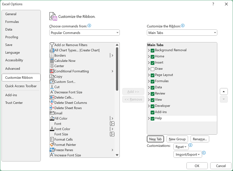
On the left you can see the various buttons and icons you can add into the Ribbon menus - and these include a few options that don't appear anywhere on the default Ribbon! If you want to easily find items to build your custom Ribbon, the top left dropdown menu has several options to help you find something useful - including "Commands Not in the Ribbon" for finding those particularly hidden gems.

On the right are the current tabs that you have. By default, this is just the always-visible tabs, but with the right-hand dropdown you can also view and customise contextual tabs, like the PivotTable tools tab, that only display under certain conditions. If we open one of these up, we can see the structure beneath:

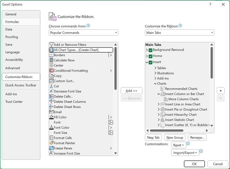
These sub-layers are 'Groups'; you can see at the bottom where you can create new groups. These groups collect items with a similar purpose - such as charts in this example. While the default tabs can't be changed, when creating your own tabs or adding items to the existing ones you can set up your own groups and pick something that works for you.

As well as that, you can use the up/down arrows on the right to reorder any custom items. New groups and tabs start with default names, but you can right click on them to rename them.

Finally, the 'Reset' and 'Import/Export' buttons at the bottom do what you'd expect - they allow you to either rest to the default tabs, or transfer Ribbon customisations between users by exporting from one machine and importing to an another.

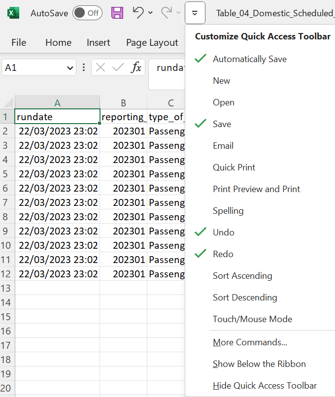
In case you didn't know, the Quick Access Toolbar is the name for the small selection of very common commands that appears right at the top left of the Excel window:

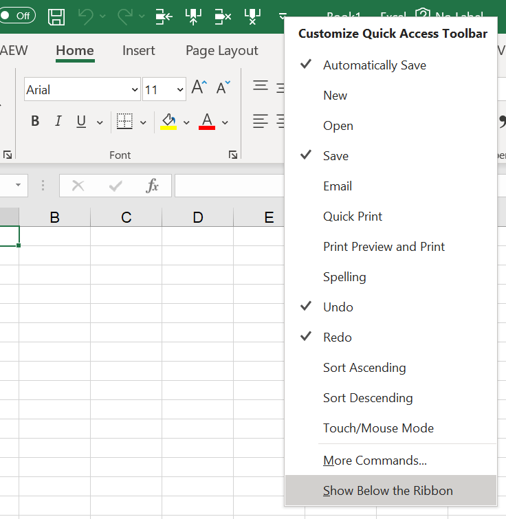
The default QAT just has autosave, save, undo, and redo. But you can amend this - either by adding some other popular commands from the small dropdown menu you see at the right there, or from the Options menu again:

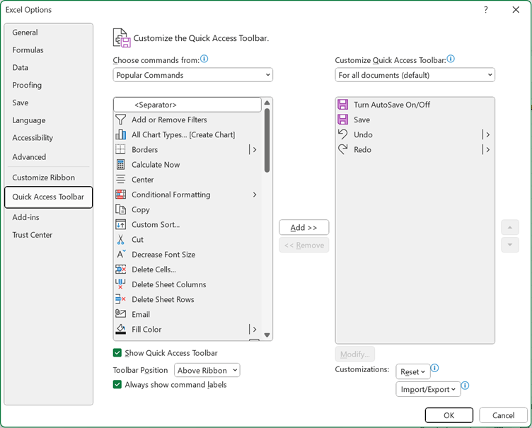
The menu and operation here are almost identical to the Ribbon customisation options above.

When combined with keyboard shortcuts changing the Ribbon and QAT can be even more worthwhile! With the default settings, Alt 2 works as a shortcut for the Save command, however many users are already familiar with using Ctrl S, so swapping it around for another command you use can be beneficial.

More on useful keyboard shortcuts for Excel has been covered in Tip #464. 

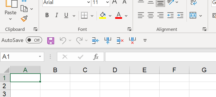
By default, the QAT sits above the ribbon as shown above. However, it is possible to move this below the ribbon which may make it easier to view and use.

The QAT looks like this when shown below the ribbon.

All in all, customising these options may not be for you - but if you have a particular set of tools or options you find yourself digging for frequently, then consider making yourself a new Ribbon tab or adding them to the Quick Access Toolbar!