Fraudulent Numbers

For example, SUM, SUMIF, SUMIFS and PivotTables are all affected by the following issue.  Consider the following summation:

In this example, the values in cells E3:E7 have been totalled in two distinct ways: the first uses SUM and the second uses the ‘+’ operator.  No difference, yes..?  Hmmm, let’s see by considering a second similar illustration:

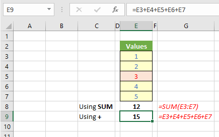
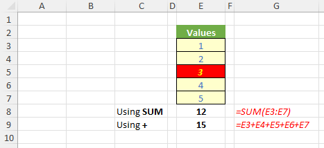
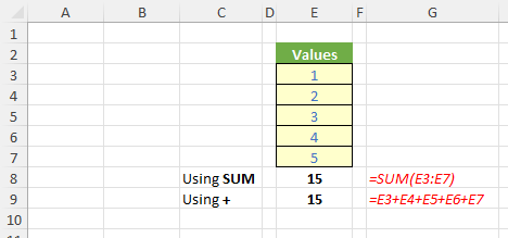
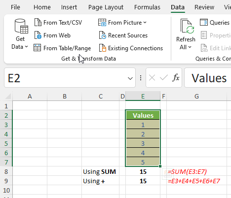
In this instance, cell E5 has been modified. It has been stored as text, even though it looks like the number three [3].  This can happen in real life when you extract data from third party management information systems and they have been stored as an incorrect data type, e.g. text.  SUM treats this number here as having zero value whereas the more convoluted addition carries on regardless because the mathematical operator ‘+’ coerces the number into behaving like a numerical value.  Multiplying by one [1] would have the same effect.  

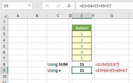
SUM, SUMIF, SUMIFS and PivotTables all treat numbers stored as text as zero in mathematical aggregations.  We need to clean the data so that the data that appears to be numerical is indeed numerical.

You might think you can spot the issue in such a small dataset, but what about the one below?

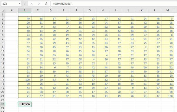
Is that summation right?  How are you going to check?  

It turns out that there is a simple way to check using the COUNT function. COUNT counts the number of numbers in a range, so we can use it to spot numbers that aren’t numbers:

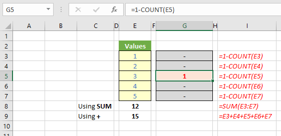
Here, the formula in column I highlights when a number is not a number.  Note how it reports by exception: if the cell in question contains a number then COUNT(Cell_Reference) equals 1 and 

=1-COUNT(Cell_Reference)

equals zero. Only non-numbers will be highlighted – it’s better to know I have two errors rather than, say, 14,367 values working correctly.

You could use conditional formatting instead:

Here, I have highlighted cells E3:E7 and then applied conditional formatting (on the Home tab, go to ‘Conditional Formatting’ and select “New Rule…’ or else use the keyboard shortcuts ALT + O + D / ALT + H + L + N).

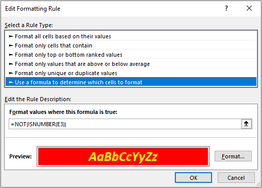
Then, I have selected ‘Use a formula to determine which cells to format’ and then typed the formula

=NOT(ISNUMBER(E3))

This calculation works on the range (ensure the cell is E3 not $E$3) in that you specify the cell in the top left-hand corner of the range selected (here, cell E3).  The function ISNUMBER is TRUE if cell E3 contains a number and FALSE otherwise. NOT then simply applies the logical opposite. Hence, any “fraudulent numbers” will be TRUE and the conditional formatting will be applied.

Great. So now fraudulent numbers are identified, how do you fix them?

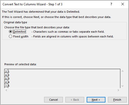
The easiest way is perhaps a little non-obvious (new word I have just made up) if you have not seen this trick before. You use ‘Text to Columns’!

For those not familiar with this age-old feature in Excel, ‘Text to Columns’ is found on the Data tab of the Ribbon and splits text in a single string into one or more columns based upon the occurrence of a special character (known as a delimiter). Comma separated value (CSV) are one such example, whereby strings are split each time a comma “,” appears.

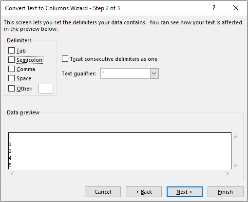
We don’t care about splitting the text, but we shall still use this feature. Let’s select the cells E3:E7 and then apply ‘Text to Columns’ (click on the button in the Data tab or use the shortcut ALT + A + E).  The following dialog will appear:

We select the ‘Delimited’ option and then click on the ‘Next’ button:

Uncheck all delimiters (i.e. the text may no longer be split). Then, rather than click on the ‘Next’ button, simply click on ‘Finish’. Lo and behold, all numbers that appeared to be values are values, viz.

Nice trick, eh?  Sometimes, for reasons I have never quite fathomed, this method fails.  If you are unlucky and this happens to you, there are two fallback options.

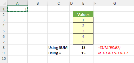
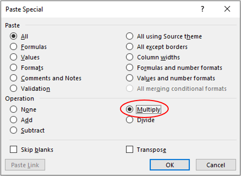
The first is a simple trick with ‘Copy’ and ‘Paste Special…’. As mentioned earlier, multiplying text that looks like a number by the numerical value of one [1] will convert – coerce – this number into its displayed value. Therefore, If I type the number one [1] into cell A1 (say) and then copy this value / cell (CTRL + C):

Next, select the cells E3:E7 (i.e. the cells we wish to paste into), and then bring up the ‘Paste Special’ dialog (go to the Home tab and from the ‘Paste’ menu, select ‘Paste Special…’ else use the keyboard shortcut CTRL + ALT + V or ALT + E + S):

Here, select ‘Multiply’ as the ‘Operation’. This has the effect of multiplying each of the destination cells by one [1], i.e. converting the numbers to numbers. At this point, you may now delete the value in cell A1 since it has now served its purpose.

Finally, don’t forget Power Query / Get & Transform. As an Extract, Transform and Load (ETL) tool, this is exactly what it’s there for.  To use this tool, select cells E2:E7 (i.e. include the header as well). Then, from the Data tab on the Ribbon, in the ‘Get & Transform’ grouping, select ‘From Table/Range’, viz.

You will be prompted to create a Table:

If you forgot to select cell E2, here is your reprieve because you may check / uncheck the ‘My table has headers’ checkbox accordingly!

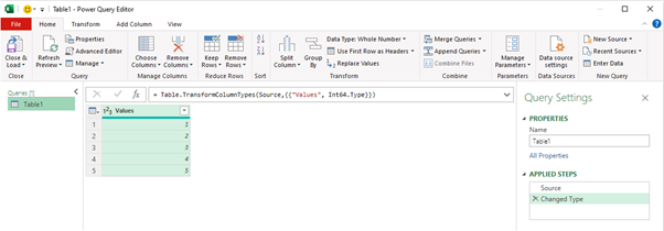
The Power Query Editor will then load, and you should note that as part of the upload, ‘Changed Type’ has automatically been applied in the ‘APPLIED STEPS’ pane and you can see here that the Data Type ‘Whole Number’ has been adopted:

By clicking ‘Close & Load’ on the Home tab of the Ribbon, the numerical values will be deposited back into Excel:

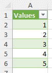
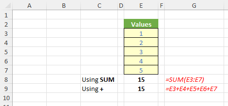
The issue with this approach is that makes a copy of the table elsewhere in the workbook and does not transform the original values (which may or may not be what you want).  Nonetheless, fraudulent numbers begone!

Word to the Wise

I strongly recommend that you apply the transformations in the order documented above.  ‘Text to Columns’ takes seconds to implement and usually works.  When it doesn’t, ‘Copy’ and ‘Paste Special…’ is a straightforward alternative, but you risk the danger of forgetting to delete the helper value [1] upon completion.  Power Query is very powerful, but it makes a copy of the data.  With large datasets, this may therefore be an inefficient solution.