Your Questions Answered #1 - How can I make custom number formats generally available?

Your community needs your questions. Please send as many as you can to us at: excel@icaew.com

Following the recent webinar, I have followed the demonstration of creating a custom number format and it works perfectly in the worksheet in which I created it. How best do I make it as easy as possible to apply and also make it available in all my workbooks?

In the recent webinar Excel tips and tricks live - your questions answered one of the questions concerned controlling the display of zero values. Presenter John Tennent demonstrated the use of a Custom Number format to control the three main types of value: Positive, Negative and Zero.

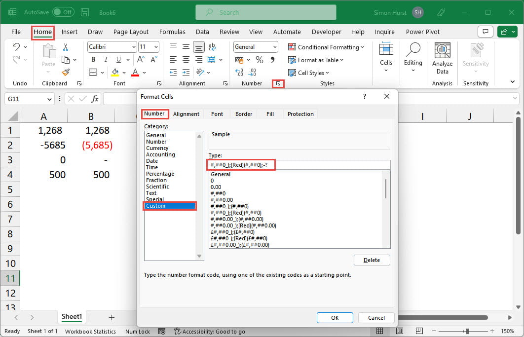
The format is created by entering special characters in the Custom section of the Number tab of the Format Cells dialog:

In this example, we have set up our three sections, separated by semi-colons, to show numbers using a comma as a thousand separator, with no decimal places. Negative numbers are shown in red with round brackets, and zero values are shown as a dash, followed by a space. Note that the positive number format ends with _). The underscore causes Excel to leave an amount of space equal to the width of the following character. So, _) leaves a space at the end of a positive number that matches the width of the closing bracket at the end of a negative number, ensuring that positive and negative numbers line up exactly:

#,##0_);[Red](#,##0);-?

Having created your perfect number format, you could apply it by going back to the Format Cells dialog, Custom category and selecting your format which will be towards the bottom of the list of formats. However, this is obviously quite a laborious process and would not be obvious to anyone else using your spreadsheet.

We will address the first part of our two-part question first: how do we make the format easy to apply?

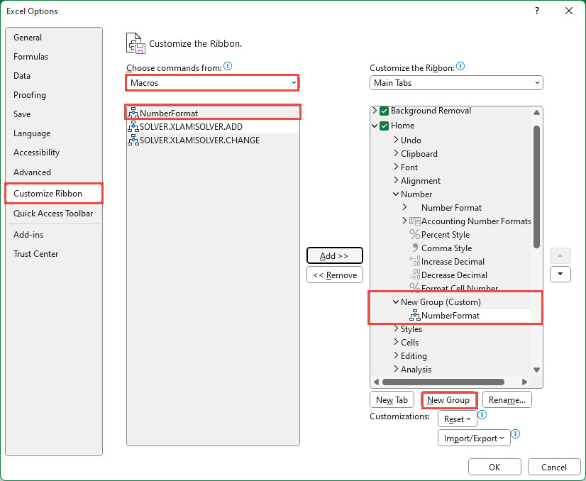
We could record a macro that applies our number format to the currently selected cells. We could then add a button to run that macro either to our Quick Access Toolbar or to the Ribbon. In either case, we right-click on the toolbar or the ribbon and choose the appropriate Customise option - we can choose whether to add our button to the toolbar or the ribbon. For the Quick Access Toolbar, we can choose Macros from the ‘Choose command from’ dropdown and then Add our new command to our toolbar. The operation is slightly more complicated for the ribbon because we can only add commands to custom groups, so we would need to create and name a new group in the appropriate ribbon tab first, before adding our command in the same way:

Depending on whether we saved our macro in the current workbook or in the Personal Macro Workbook, this command would work just when the current workbook is open or throughout Excel. The Personal Macro Workbook is a hidden workbook that is opened whenever Excel is opened, making any macros that it contains generally available.

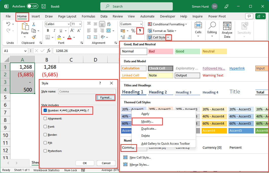
If you would prefer to avoid the use of macros and programming code, there is a very quick and easy method to make the new format available in the current workbook. It involves using Cell Styles. Excel Cell Styles are found in the Styles group of the Home Ribbon tab and, at the bottom of the gallery of styles is group of Number Format styles, including a Comma format. This Comma format number style is linked to an existing Ribbon tab command: the Comma button in the Number group of the Home Ribbon tab. Accordingly, if you right-click on the Comma style in the Style Gallery and choose Modify, you can use the Format button to display the Format Cells dialog from which you can choose your custom number format to replace the existing comma number format. Having modified the Comma style in this way, you can apply your format just be selecting the relevant cells and clicking the Comma button:

As effective and easy a solution this is for the current workbook, it doesn’t solve the problem of applying the format in other workbooks.

How do make the format available in all my workbooks?

Unlike Word styles, Excel styles cannot be made directly available to all workbooks. If you have allocated your number format to your Comma style then, if a workbook is open that includes the style, you can use Merge Styles… to copy styles from that workbook over the existing styles in any other workbook. Note that any cells that have previously had the Comma style applied will then automatically change to use your custom number format.

There is a way to make your custom number format style, and its allocation to the Comma button, available to all new workbooks. You can add the style to an Excel template. If that template is saved with the name Book.xltx into the User StartUp folder (taking care not to overwrite an existing file) then your template will be used as the default template when creating a new workbook and your Comma button will apply your custom number format in all new workbooks: ICAEW 20 Principles Excel workbook template

• Accountants' guide to Excel - mastering number formats part 1 (2023 update)
• Accountants' guide to Excel - mastering number formats part 2 (2023 update)