Excel Tip of the Week Live Q&A 5 - ALL your questions answered

Is it possible to create a consolidated pivot table from multiple excel sheets in the same file?

There are a couple of ways of consolidating data like this. Firstly, you can use Data => Consolidate and manually select each data range.

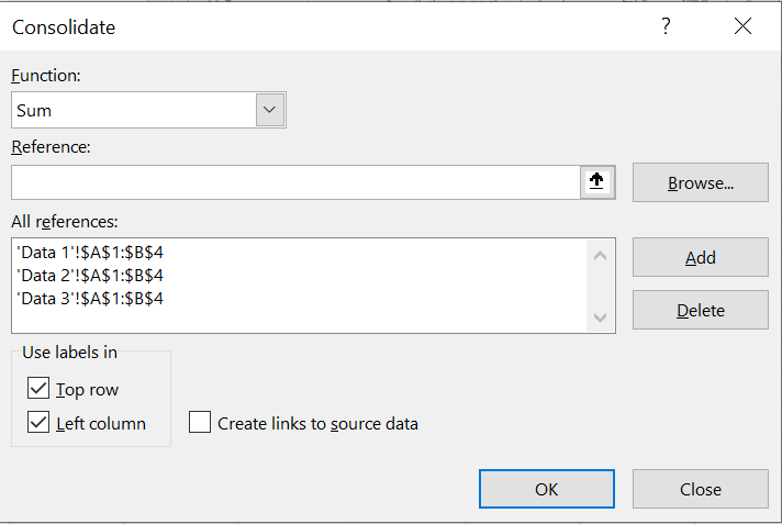
However this is a very manual process and won’t update if the source data is updated.

Secondly, you could add each dataset to the data model using Power Query (Data => From Sheet), and then create a new query that appends all of these into one. This will update if refreshed. See our other webinars on PQ for more details.

Is the consolidation able to reference the names of the tabs Mon, Tue, Wed?

No, you would need to add this as a manual column.

Could you please give a recap of the XLOOKUP function?

XLOOKUP is a new lookup function in the latest Excel versions, which is a superior replacement for VLOOKUP or INDEX MATCH if you’ve been using those before. The syntax is:

            =XLOOKUP(lookup item, row or column to search in, data to return, [optional value to use in case the lookup item is not found])

A simple one to start - how do I quickly convert US dates with a "." separator, to UK format?

Sadly not as simple as you might like.

You need to separate the input data into separate day, month, and year, and then use the DATE function to reassemble them into a single, correctly-formatted UK date. You can do this process using Text to Columns, find & replace, or using formulas such as LEFT, RIGHT, and MID (possible combined with FIND if the different elements aren’t consistent in length). See the file for some examples.

Watch out for any cells that have already been formatted by Excel as dates – e.g. 04/05/2021 is valid in either format; a US dataset might have intended “April 5^th”, but UK Excel will read this as “4^th of May”. In these cases you need to use a formula such as:

            =DATE(YEAR(A1), DAY(A1), MONTH(A1))

I am interested in actuarial functions, such as IRR, PV, FV…

Is there anything you can show us how to watch out for putting in correct values and dealing l with error checking in IRR, PV, FV?

These are useful functions and most – PV, FV, NPER, RATE, and PMT – are easy to learn as a batch because they all use consistent terminology. Check out our TOTW blog on the subject.

The main pitfalls with these functions is that a) you must be consistent with time periods – e.g. don’t mix annual interest rates and monthly payments; and b) the present value and any payments must have opposite signs.

NPV and IRR are simpler, but it’s important to understand the date basis they use. NPV discounts the first value one tick, for example, meaning that any day-0 amounts need to be added outside of the function. See TOTW #169 for details.

Can we have interactive dashboards similar to Google Data Studio?

You can make dashboards in Excel, but they are much more manual.

Is it possible to have double-clicking on a data cell in a Pivot Table show the data flat (as it was until ....) and NOT in a "Table"

Unfortunately not. I don’t recommend leaving these snapshot reports in a workbook long-term as they aren’t “live” connected to any data, so they can be misleading.

Can you remind me how you can change a whole table/row/column from Capital to small letters and vice versa?

In Word, Shift F3 does this, but in Excel you need to use the UPPER / LOWER functions in a separate row or column of cells, and then copy & paste values over the original data.

Is there a shortcut to update formulas in highlighted cells without the whole tab or spreadsheet?

If you select only the specific cells, you can type the new formula in one of them, then press Ctrl Enter to adjust them all. Or use Data => Filter to show only the specific cells before making the change.

We have given access to an excel reporting file to a mac user. It reports on productivity by merging time entries from different reports. The data is updated manually by copy/paste into separate tabs within the file, which then go up into power query and the output comes into pivot charts and tables. The mac user cannot see the size of the tables (does not have the resize option) or refresh the power query which uses them. Are you aware of any mac compatibility issues with excel - both sides use office 365 - or is there a basic setting which we could be missing? There are no external connections, the file is standalone.

Unfortunately Excel for Mac has only recently gotten Power Query at all, and it’s less fully-featured than the Windows version, so at a guess that’s likely the issue.

Is there an efficient way of formatting data labels (e.g on top of the bars on an histogram), instead of selecting each one individually?

If you right click one of them, you should see “Format data labels”, from which you can access a sidebar menu that will format all of them.

I have problems setting up Pivot tables:

a) problems in in deciding what should be column headings and what should be rows

This is really down to preference, but generally I would recommend for ease of reading that fields with lots of variables go into rows and ones with only a handful use columns.

 b) Could you show me how to manipulate the filter and using totals and sum totals?

You can filter items in PivotTables from four places:

1. Filter which rows are included in the Pivot at all using a field in the “Filters” area
2. Filter row labels from the dropdown at the top of the row labels
3. Filter column labels from the dropdown at the left of the column labels
4. Filter the values themselves using either dropdown from b) and c), and selecting “Value filters”

You can choose which totals and subtotals to include in the Pivot from the PivotTable Design menu.

c) Any new things that have come in to the filter of pivot tables?

Nothing lately, no.

Is there a way to identify which numbers (out of many numbers) give a certain grand total?

Can you explain what I can use Solver in what would be inputs and outputs using an example?

This is called the “subset sum problem”. There’s no algorithm for perfectly doing it, but you can automate the process using the Solver add-in. We covered this in TOTW #365.

Can you show steps to convert data from pivot tables to charts and graphs? What problems could I foresee in setting them up?

The main thing is to be careful about which summation option you choose. When you add a field to a PivotTable, it will automatically choose to either sum or count it based on the content – but you might want to do something different to what the default is.

How can you change a name so that the surname is before the given name?

It is possible to do this using a complex formula:

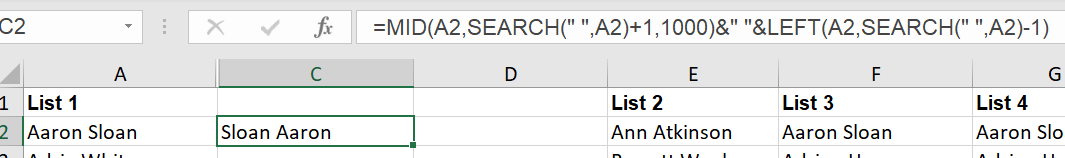
However, this is much easier to do by typing the value you want for the first item, and then using Ctrl E or Home => Flash Fill. This will have Excel use AI to figure out the change you want and then automatically do the same for the rest of the column.

Note that for names specifically there is no perfect answer – people can have multiple word given names and multiple word surnames, as well as middle names or initials, so watch out for errors.

In PivotTables, I find myself repeatedly using Pivot Table Options > Display > Classic Pivot Table Layout. Is it possible to set something somewhere so that this happens for every new table I create?

This is possible in Excel 2019 and up, from File => Options => Data => Edit Default Layout. It will apply prospectively to any new Pivots you create, but won’t affect any that you have already created.

Setting up a PivotTable so that some items are filtered out, but new items ARE included requires: Field Settings (double-click on the fieldname) > Include new items in manual filter. Is is possible to set something somewhere so that that box is defaulted to ticked for ever new table I create?

This one unfortunately I don’t believe can be made a default.

Is there a webinar or part of webinar that covers conditional formatting? It never seems to work as smoothly as you think it should (for me anyway!).

Yes, we have covered it in several of the “Excel Tip of the Week Live” series, found here.

Is it possible to create a "paste values" icon?

Yes, you can right click the Quick Access Toolbar (right at the top of Excel) and customise it from there to include any item, including a Paste Values button.

In a large spreadsheet on a big screen, is there a setting which highlights the whole column and whole row relating to the active cell I'm in?

Not continually, but you can use Ctrl Space or Shift Space for a quick orientation.

For copy and paste, can we keep the original formula (with cell) without auto changing?

Normally when you copy and paste a cell with a formula in it, any cell references in that formula are amended to match – e.g. if you paste one column to the right and three rows down, the cell references in the formula are also moved one column to the right and three rows down.

If you don’t want a cell reference to be changed when a formula is pasted, you need to write it with dollar signs. Write $A$1 for a reference that shouldn’t be changed at all, $A1 if only the column part should be fixed, and A$1 if only the row part should be fixed.

Where I have a large spreadsheet with formulas and I set the spreadsheet to manual calculation, I would like to refresh the formula on a set of selected cells without the whole spreadsheet.

Excel’s inbuilt recalculation engine already does this (only recalculating what’s needed), so just using a refresh should work

How did you get the formulas to be visible in the cell during the live demo?

The newer function FORMULATEXT.

Excel has a new LAMBDA function (live or coming out soon) where you can assign your own formula / function to LAMBDA. Do you have examples of how this might be used in practice - not so much the mechanics of writing the formula, but the context of where this might be deployed in a way that makes modelling / reporting easier / more flexible / robust? i.e  how will LAMBDA actually improve how we do things & structure workbooks over existing formulas?

I think LAMBDA is a little early-days as of yet, but I currently view it like User-Defined Functions in VBA – sometimes useful, but they do add a lot of opacity and complexity to your workbooks. LAMBDA is particularly useful for making your own calculations where you need iteration or self-reference, but really the main takeaway for now is to try and avoid needing them if you can make a simpler workbook instead.

In a PivotTable, can you sort by a subtotal (such as a customer total in a list of invoices) and then also produce a pivot table of the top 10 Customers?

Yes, you can sort according to anything by selecting a cell with that value in it and then using Data => Sort.

The filter options (explained above) for rows or columns allow for custom filters like “Top 10”.

If you have several criteria as rows in a pivot table what is the best way to format the table to show the subtotals, as I struggle with formatting the tables differently.

It’s down to individual preference, but many people like to use the “tabular” layout (from the PivotTable Design menu), or the default Compact layout. It really depends on what your data looks like and what you’re trying to do.

How close is Goal Seek to the Solver add-in?

Very similar – it’s basically a simpler Solver. Goal Seek can modify only one input cell and can only attempt to get the target cell to a specific value; Solver can modify multiple input cells, can have additional constraints added to it, and can find a maximum or minimum value instead of just trying to hit a specific target. Goal Seek is quicker and easier to use where it is sufficient, though.