Pro-rating hours in a month

As you may probably imagine, in such hallowed climes several solutions were pitched, but many required the use of LET, LAMBDA, dynamic arrays and Power Query. These functions, features and tools simply aren’t available in every version of the spreadsheeting software. I decided I wanted to derive an answer that would work in all versions of Excel. See what you think.

The attached Excel file hopefully clarifies my suggestion too.

Consider the following dataset:

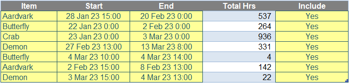
I have several projects (or Items) that are live and that are being charged to (sometimes with overlap). I simply want to know how many hours are being worked each month for each Item, assuming the hours recorded should be included (through observing whether the value is “Yes” or otherwise in the "Include" column).

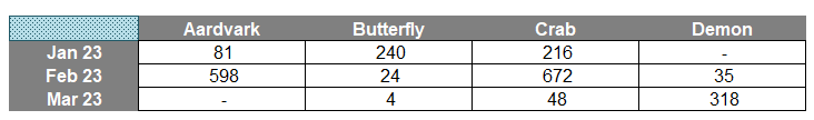
The summary should look as follows:

Summary table

The question is, what formula can be written that may be copied down and across the whole table that will work in all versions of Excel? 

Before I discuss my solution, I’d like to note there are several complicating factors here. Let’s go through them.

Problem 1: Anchoring References in a Table

First of all, I am going to assume that the dataset has been created as an Excel Table (by selecting the range and then clicking on "Table" in the "Tables" group of the "Insert" tab of the Ribbon, or by using the keyboards shortcut CTRL + T), and that this Table is called Example.

If I were to create a formula to highlight the data in the Start column of the Example Table (i.e. selecting from 28 Jan 23 15:00 through 3 Mar 23 15:00), I would get the equation

=Example[Start]

i.e. select the data in the field Start in the Example Table. However, if I were to copy the formula across one column, the formula would change as follows:

=Example[End]

Do you see what has happened? Copying across a column moves the reference one column to the right to the field End rather than remaining on Start. We need to anchor the reference and the dollar ($) signs normally employed in Excel will not work here. In this instance, you must manually adjust the formula before copying as follows:

=Example[[Start]:[Start]]

This double reference to the field Start has the effect of anchoring the field. If you don’t know this trick, it’s well worth knowing.

Problem 2: Calculating the End of a Month

Our first issue is overcome, but there are more. Let’s now consider working out the end of the month – which is essential in working out how many hours are charged to each month. Many of you will know that EOMONTH provides you with the end of the month. This function’s syntax is as follows:

EOMONTH(start_date, months)

The EOMONTH function has the following two [2] arguments:

• start_date: this is required and represents the start date. Dates should be entered by using the DATE function, or as results of other formulas or functions. For example, consider using DATE(2023,5,21) for the 21st day of May, 2023. Problems can occur if dates are entered as text
• months: this is also required. This represents the number of months before or after the start_date. A positive value for months yields a future date; a negative value yields a past date.

Thus, EOMONTH(date, 0) calculates the end of the month date resides in, yes? Er, yes and no. Allow me to explain. Consider:

=EMONTH(DATE(2023, 5, 21), 0)

The argument DATE(2023, 5, 21) generates the date 21 May 2023. Therefore, EMONTH(DATE(2023, 5, 21), 0) calculates the end of the month 31 May 2023. So it’s a “yes”, it does generate the end of the month.

No.

If you format the resulting date accordingly, you will see the formula has resulted in

31 May 23 0:00

This means it is at midnight on that day and there are still 24 hours to go until the end of the month. Therefore, for our problem to calculate the last moment of a month we will have to use formulae similar to

=EOMONTH(date, number_of_periods) + 1

It is a common mistake modellers often make – don’t fall into this trap!

Problem 3: Restricting the Start and End Times

The next issue is restricting the start and end times. To work out the overall duration (in days), the formula is simply given by

=End – Start

Not much of a complication there, Liam. However, when you try to restrict this to a particular month it gets more complex. We only want to consider the relevant time for that month. For example, if End occurs after the end of the month then we will wish to restrict it to the month end. Similarly, if End occurs before the start of the month, we would wish to ignore it, which can be done by assuming it occurs at the start of the period (so the time cannot be greater than zero; this avoids negative values being considered too).

The first condition equates to:

=IF(End > Current Month End, Current Month End, End) or
=MIN(Current Month End, End)

Similarly, the second condition equates to:

=IF(End > Prior Month End, End, Prior Month End) or
=MAX(End, Prior Month End)

Combining these two conditions you get:

=IF(End > Current Month End, Current Month End, 
IF(End > Prior Month End, End, Prior Month End)) or

=MIN(Current Month End, MAX(End, Prior Month End))

That’s just for the End date! Similar logic will obtain

=IF(Start > Prior Month End, 
IF(Start > Current Month End, Current Month End, Start), Prior Month End) or

=MAX(MIN(Start, Current Month End), Prior Month End)

The total hours for the month would then be given by

=Restricted End – Restricted Start

= MIN(Current Month End, MAX(End, Prior Month End)) 
– MAX(MIN(Start, Current Month End), Prior Month End)

One of my favourite tricks when you have restricted upper and lower bounds is to use the MEDIAN function. This idea was shown to me by fellow Excel MVP Brad Yundt and is rather clever – and yet irritatingly simple. As a reminder, the MEDIAN function determines the middle number of a group of numbers when placed in order. Therefore,

=MIN(Current Month End, MAX(End, Prior Month End))
=MEDIAN(Prior Month End, End, Current Month End)

Similarly, 

=MAX(MIN(Start, Current Period End), Prior Period End)
=MEDIAN(Prior Month End, Start, Current Month End)

Therefore, our restricted total hours for the month may be simplified to 

=MEDIAN(Prior Month End, End, Current Month End)
– MEDIAN(Prior Month End, Start, Current Month End)

This is a great trick for these sorts of problem and is included here for consideration. Unfortunately, due tour fourth issue, it’s not going to help us here…

Problem 4: Summing Ranges

Our issue here is that we have more than one row of data. Using Excel 365 (which will not be necessary for my proposed solution) allows me to use dynamic arrays, which will demonstrate the next problem. Consider the following:

In the above illustration, in column G, I have linked to the data in the Start field of my Example Table. In column H, I have similarly linked to the End field of my Example Table. Column I (formatted as days) has been generated by highlighting cells H36:H42 (which results in the reference H36#, meaning the spilled range starting in cell H36) and then subtracting of the spilled range G36#. This gives me End – Start with no restriction on a row by row basis.

Problems occur when I try to use some functions in Excel with ranges / arrays. Let’s imagine I just wish to restrict column H so that it cannot exceed 31 January 2023 (which would be calculated as EOMONTH(DATE(2023, 1, 31), 0) + 1):

What has happened here? The spilled range of cells H36:H42 has simply become the cell H36. This is because it has taken the minimum of all the dates in the End field and the end of the month, which is 1 February 2023 0:00, as explained earlier. This function coerces the range into one cell – it will not calculate on a row by row basis.

Similarly, the use of MAX, MEDIAN and SUM will also coerce the results, so we may not employ any of these techniques. To calculate on a row by row basis, I will have to calculate using the original longhand computation excluding all of these functions, viz.

=IF(End > Current Month End, Current Month End, 
IF(End > Prior Month End, End, Prior Month End)) 
– IF(Start > Prior Month End,
IF(Start > Current Month End, Current Month End, Start), Prior Month End)

It is convoluted and cumbersome, but it will work and will not coerce the results. This is because of how the Excel calculation engine works presently.

Suggested Solution

I am now in a position to put all my learnings together.

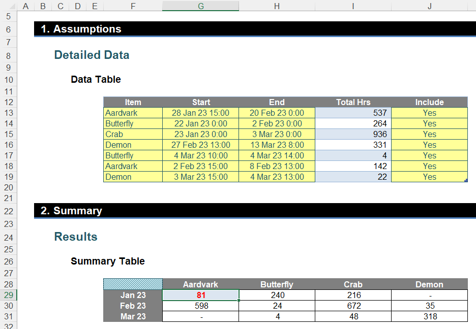
In the attached Excel file, I have constructed the following summary table. The dates in cells F29:F31 have been entered as 31 Jan 23, 28 Feb 23 and 31 Mar 23. However, as long as they are recognised as dates, the suggested solution formula in cell G29 will work:

=SUM((IF(Example[[End]:[End]]>EOMONTH($F29,0)+1,EOMONTH($F29,0)+1,
IF(Example[[End]:[End]]>EOMONTH($F29,-1)+1,Example[[End]:[End]],EOMONTH($F29,-1)+1))
-IF(Example[[Start]:[Start]]>EOMONTH($F29,-1)+1,
IF(Example[[Start]:[Start]]>EOMONTH($F29,0)+1,EOMONTH($F29,0)+1,Example[[Start]:[Start]]),EOMONTH($F29,-1)+1))
*(Example[[Item]:[Item]]=G$28)*(Example[[Include]:[Include]]="Yes"))*Hours_in_Day

This is simply the formulaic interpretation of the derived solution (above):

• Example[[Start]:[Start]], Example[[End]:[End]], Example[[Item]:[Item]] and Example[[Include]:[Include]] simply anchor the fields Start, End, Item and Include respectively
• EOMONTH($F29,-1)+1 calculates the end of the prior month
• EOMONTH($F29,0)+1 calculates the end of the current month
• (Example[[Item]:[Item]]=G$28) requires the Item to equal the value in cell G28 (the dollar sign is to anchor on the row when copied down, but allow the column to vary as the formula is copied across)
• (Example[[Include]:[Include]]="Yes") requires only items to be included to be, er, included
• multiplying by Hours_in_Day converts the total from days to hours by multiplying by 24 (this is a range name given in the attached Excel file).

Admittedly, the calculation looks horrific, but this is merely because certain references and computations have to be cited several times in the formula. Furthermore, for some versions of Excel, this formula will need to be entered using CTRL + SHIFT + ENTER rather than ENTER so that it appears in braces (the curly brackets may not be typed in), viz.

{=SUM((IF(Example[[End]:[End]]>EOMONTH($F29,0)+1,EOMONTH($F29,0)+1,
IF(Example[[End]:[End]]>EOMONTH($F29,-1)+1,Example[[End]:[End]],EOMONTH($F29,-1)+1))
-IF(Example[[Start]:[Start]]>EOMONTH($F29,-1)+1,
IF(Example[[Start]:[Start]]>EOMONTH($F29,0)+1,EOMONTH($F29,0)+1,Example[[Start]:[Start]]),EOMONTH($F29,-1)+1))
*(Example[[Item]:[Item]]=G$28)*(Example[[Include]:[Include]]="Yes"))*Hours_in_Day}

Word to the wise

As mentioned earlier, simpler variations are possible using LET, LAMBDA, dynamic arrays and Power Query. Unfortunately, these solutions will not work in all versions of Excel. The approach detailed here should work for all current variations of Excel and allows for the formula to be copied across and down as required.

Finally, this example assumes no check is needed for end times to be greater than or equal to start times and that no amendment is required if times overlap for an item – but feel free to modify the formula accordingly should you wish!