Excel Tips & Tricks #479 – Advanced Filter redux

This topic was last covered in Tip #287.

How does Advanced Filter differ from regular filters?

Regular filters add easy-to-use dropdown menus to column headings in tabular data. They are quick, effective, and easy to use. More has been covered on filters in Tip #424. So when would you use Advanced Filter?

Advanced Filter lets you write database-style queries for your data and output the rows that match. Simple queries (such as finding items where a column has a certain value, or where a column's value is between two limits) aren't particularly worth doing with Advanced Filter - the common filtering options are superior. But regular filters have one issue - they work on a column-by-column basis, and you can't create filters that simultaneously check multiple columns. If you apply filters to three columns, the conditions are always cumulative - you'll only see things that match all the separate conditions. Advanced Filter lets you make something conditional.

For example, let's say we're doing a purchases review. We might care about purchase approvals which are outside of policy - which is based on a combination of the approver ID and the amount. But the two work in combination - so we couldn't filter this data using traditional filters and would have to either do several independent filters or create a formula to help us identify the rows in question.

But we can also use Advanced Filter for this - as we'll demonstrate below.

How do you create an Advanced Filter?

We're going to create some filters for this invoice approvals data:

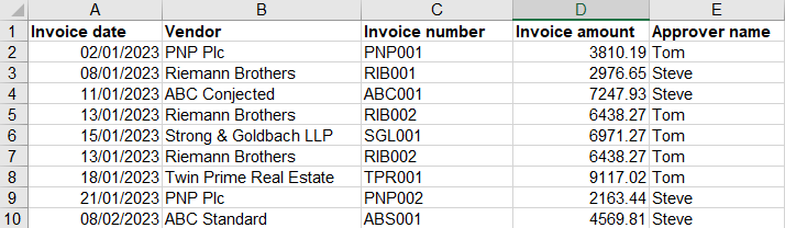
Unlike regular Filters, Advanced Filter requires that you lay out the query in the cells of the spreadsheet in a prescribed format. You have to write the column names of the columns you want to include in your filter in the top row, and then the filter conditions underneath the relevant heading(s).

For example, if we want to filter to show all the invoices from PNP Plc:

The menu here is the Advanced Filter menu, opened from the Data Ribbon. We have told Excel the locations of the "list range" (where the data is) and the "criteria range" (our filter condition(s)).

Note that there are a couple more options than with normal filters:

1. We can choose to copy the list of matching items to a given location instead of just filtering.

2. We can choose to show only unique records if duplicates exist.

How can you create more complex filters?

The basic rules for building up your Advanced Filter are:

1. You can apply conditions to more than one column by adding more columns to your criteria range.
2. Conditions that are all on one row are additive - the data will have to match all of them to be shown.
3. Conditions on different rows are options - the data can match either and still be included in the filter.

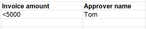
So, for example, here's the criteria range for "Invoices above £5,000 that were approved by Tom":

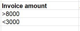
And here's the criteria range for "Invoices that are either above £8,000 or below £3000":

Note the use of < and > for inequality-based conditions. You can also use <> for "not equal to".

Here's our final example - a test to find any invoices where approves exceeded their approval thresholds:

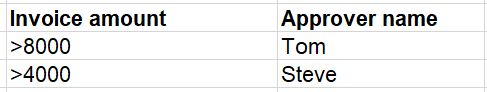
This allows us to quickly identify all exceptions to the approvals policy with a single filter and no formulas.

It’s important to remember that to find rows that meet multiple criteria in multiple columns (e.g., where a AND b must be true), you must type all the criteria in the same row of the criteria range.

Conversely, to find rows that meet multiple criteria in multiple columns where any criteria can be true (e.g., where a OR b can be true), you must type the criteria in the different columns and rows of the criteria range.

Using wildcard criteria

Wildcard criteria can be helpful to find text values that share some characters but not others. There are three wildcard characters in Excel that can be used in the criteria range:

1. ? (Question mark) – represents one single character. For example, T?m could mean Tom or Tim.
2. * (Asterisk) – represents any number of characters. For example, ex* could mean excel or example, and *east could mean Northeast or Southeast.
3. ~ (Tilde) – is used to identify a wildcard character (~, *, ?) in the text.

For example, to search for both “Tom” and “Tim” in my approver name list, I can enter =”=T?m” under approver name. The wildcard criteria must be entered in that format.