Leveraging maths and stats in Excel for deeper data insights - part 1

As a finance function, we are often presented with vast quantities of data – how can we use the statistical capabilities within Excel to extract useful insights? Following on from the successful webinar on this topic, this series of articles will explore practical applications of maths and stats functions in Excel.

Four key principles to start with:

The past does not predict the future – Whilst we can derive trends and patterns in our historic data, the extrapolation of these to predict future values is unrealistic.  No data forecast saw the pandemic or oil price doubling in 2022.  What we can do is use maths and statistics to add to the decision-making process not replace it.

Unnecessarily searching for a single point forecast – Many people spend too much time trying to identify a single future value when the task is simply impossible.  We can be much more effective identifying a range where the forecast may lie and then understand the implication of being at various points within that range.  Take for example inflation - What will it be next year?  Trying to ‘guess’ the number to one decimal place is futile.  Why not identify a range where it might fall. Perhaps 5% to 10% and see what the implications to the business might be of being at the ends and middle of that range.

Avoid spurious accuracy – In 1982 A.S.C. Ehrenberg wrote a book titled ‘A Primer in Data Reduction’ to help us make sense of the increasing amount of data that computers were capturing and storing.  In his book he asserts that you only need two digits (significant figures) to make a decision.  For example, if you had a project that could generate £1.4m you would not make a different decision if you knew it to be £1.43m.  Therefore, describe the future with indicative numbers not detail.

Only use Maths functions you can explain to others – In Excel there are many wonderful maths and statistics functions and features.  However, only use the ones you understand and are confident provide the information you require.  Ensure you can explain the basis to anyone who asks about the values generated.  My view is only use a function that you can explain and can explain without reference to notes.  If you need notes, you are not close enough to what is really being calculated.

With these principles in mind, we can have an effective exploration of the really helpful maths and statistics functions available to us.

The series will develop as follows:

1. The introduction, setting up Excel and essential analysis techniques
2. Forecasting – both moving averages, weighted averages, and exponential smoothing
3. Regression – trend lines and equations for forecasting
4. Day counts and calendarising seasonal data
5. Bass diffusion curves to forecast future volumes and market shares
6. Normal distribution curves and probabilities of success

Screen shots will be from Excel within Microsoft 365.

The example we will use in the first two blogs is to understand the sales pattern of a product.  In this case milk in a corner shop.  By identifying if demand is rising or falling, we can manage our supply more accurately, potentially avoiding both waste and being out of stock.

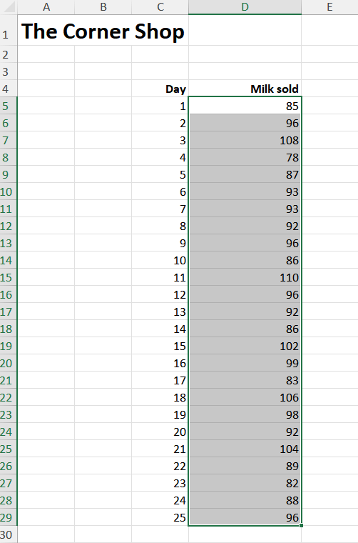
The range highlighted is D5:D29 showing sales data over the last 25 days. This will be used in the calculations below.

Customise your Status Bar

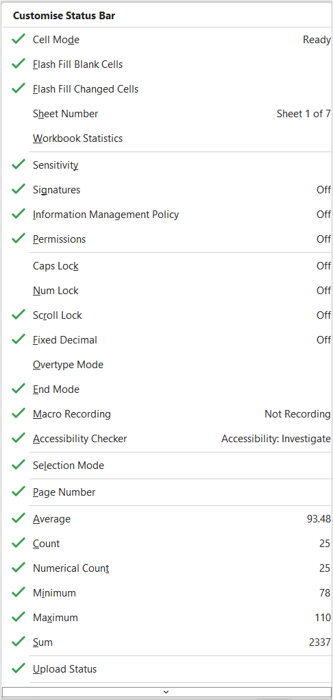
At the bottom of the Excel screen is the Status Bar, the right-hand end of which has the Zoom in/out slider.  On this Bar you can display a few basic attributes of a range.

Average – average of the numbers in the range
Count – number of cells in the range that are not blank
Numerical Count – number of cells in the range containing a number 
Min & Max – the highest and lowest values in the range
Sum – the total of the numbers in the range

Excel default is normally to have the Sum visible and you have to enable the other attributes.  To do this right click the Status Bar and the following options appear – select those you want enabled.  These numerical ones are at the bottom of the list.

Essential Analysis

=AVERAGE(Range) – This will calculate the average of the range but beware any zeros in the range will be counted as values. Blank cells are omitted. Therefore, be careful how missing data is represented.

=COUNTA(Range) – This will return the number of cells in a range that are not blank

=COUNT(Range) – This will return the number of numeric values in a range

=MIN(Range) and =MAX(Range) – The smallest and largest values in a range

=SUM(Range) – The total of the range

Two other useful functions are:

=Median(Range) - When sorted in order it returns the middle value. If there is an odd number of items, then it is an actual value. If there is an even number of items, it is the average of the middle two items.

=Mode(Range) - The most frequent value. If the range is just single instances of values, the result is N/A. If there are two or more items with the most frequent value, then the first of these in the range will be shown.

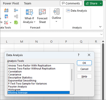
The Analysis ToolPak

Within Excel is an additional set of statistical functions that can be accessed through the Analysis ToolPak. We will explore the application of some of these in blog 2, such as moving averages and exponential smoothing. In this blog we will show you how to get the Add-in up and running.

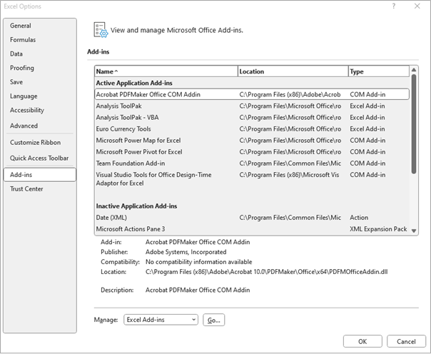
The Analysis ToolPak is available within the standard Excel package, all that you need to do is enable it (switch it on). To do this select the File Ribbon and down the left of the screen is the menu of items.  Select the one at the bottom of the screen titled ‘Options’. In the next dialog box, there is also a menu of items down the left-hand side.  Second from the bottom is ‘Add-ins’, click on this.

The Add-ins will appear and down the bottom of the screen beside the word ‘Manage’ is a drop-down menu. Select the words ‘Excel Add-ins’ and press the button Go…

In the next dialog box click the small square box to the left of the word Analysis ToolPak and a blue tick will appear.  Press OK and the Add-in will be enabled.

Once enabled the ToolPak can be accessed from the right-hand end of the Data Ribbon.  You will see a new Group titled Analysis and within that an icon for Data Analysis.  Press the item and a new dialog box appears with a list of all the Analysis Tools that can be applied with this Add-in.

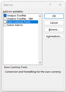
Should you later decide you didn’t want this Add-in running within your Excel, it can be removed in the same way as it was added.  Just click the Blue tick in the Add-ins dialog box and the tick will disappear.  Once OK is pressed it will be removed.

In the next blog we will continue to use the milk example and we will apply a moving average, weighted averages, and Exponential smoothing.  The benefit of using the Analysis ToolPak is that it not only does the calculations for you, but also draws charts too.