#453 – Revisiting Audit Sampling with Dynamic Arrays

A reminder on Dynamic Arrays

If you’ve not come across dynamic arrays before – where have you been?! For those readers who have been living under a rock, dynamic arrays are a relatively recent addition to Microsoft Excel that allow formulas to “spill” their output across multiple cells. The “dynamic” element means Excel adjusts the range of the output based on the range of the input – transforming standard formulas automatically. For more, do take a look at the related links at the bottom of this post.

Sampling Template

At the heart of this post is a template Excel file which we’ll talk through below:

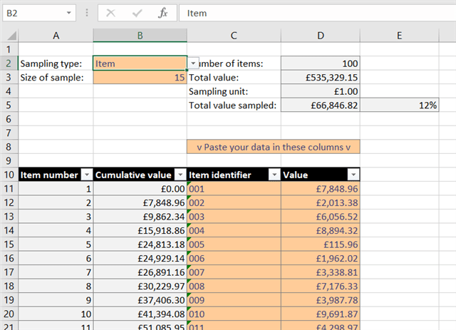
The options at the top allow the user to specify whether they want item sampling (in which all items have an equal chance of being chosen), or monetary unit sampling (in which the sample is weighted towards the larger items). They can of course also specify the size of the sample they want.

The lower part of the template is an Excel Table, which allows the formulas used in the sample selection to automatically adjust based on the size of the population that the user pastes into the table. In this example, we have pre-filled the template with a 100-item population.

There is also a cumulative total column that is calculated automatically by formulas, that we will be using for the monetary unit sampling later on. This shows the total of the items prior to the current line.

The formula for this column is:

=SUM(INDEX([Value],1):[@Value])-[@Value]

In short, this defines the SUM range as being from the first row in the ‘Value’ column, to the current row (designated by the “@”). See TOTW #201 for more on the INDEX function. We then subtract the current row's value to show the total prior to the current row.

The other items in the template are calculated automatically. “Number of items” and “Total value” are both relatively self-explanatory. "Sampling unit" shows the size of monetary units that are used if the “Monetary” sampling type is selected. The calculation is:

=10^IF(D3<1000000,0,ROUNDDOWN(LOG10(D3)-5,0))

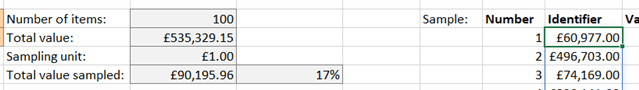
Essentially this will use a unit of £1 if the total items have a value of £1,000,000 or less, and otherwise will choose a power of 10 based on the size of the sample desired. This is necessary because of the way the monetary sample is calculated, and prevents the dynamic arrays that Excel creates in the background from exceeding the standard row limit of 1,048,576 items.

Building our formulas

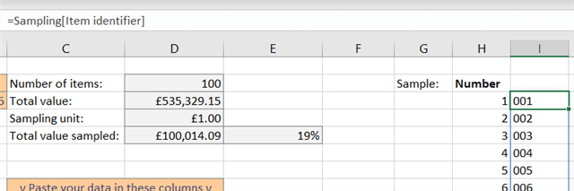
First off, we'll create a numbering for our sample. This is just a SEQUENCE function that looks at the size of the sample selected and populates a number of rows based on the input:

=SEQUENCE(B3)

This isn't just neat labelling - we will also use this SEQUENCE function to control the number of items that we return from our random sampling process later on.
The key formula is the one which returns our sample of identifiers in column I; this is built from two formulas based on whether the user selects Item or Monetary Unit sampling. For this post we'll build up each separately as an example.

Item sampling

Here what we need to do is:

1. Bring in our list of (in this case) 100 items.
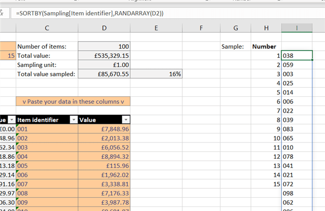
2. Sort the list into a random order.
3. Pick a number of items from the top of our random list that matches the user's desired sample size.

Let's look at each of those stages and build up our dynamic array formula step-by-step. First, listing all off the items:

This is just a matter of referring to the identifier column of the Excel Table - the list will automatically spill into the following cells. Next, we need to randomise this list. To do this, we are going to make an array of random numbers the same size as the list in the table, and then sort the list of identifiers according to that random list. To do this we use RANDARRAY to make the random numbers, and SORTBY to use that as the sorting key for the item identifiers:

This gives a shuffled-up list of all 100 items. Finally, we need to pick just the first few items in this list, to match the chosen sample size. To do this, we are going to use an INDEX. Normally INDEX will pull the nth item from a list - so e.g. =INDEX(array, 1) would pull the 1st item. However, in our case, instead of using 1, we'll point at our SEQUENCE function using the new #-style referencing. This will create a spilled function that will take the 1st, 2nd, 3rd and so on items from our shuffled list, and return each in turn.

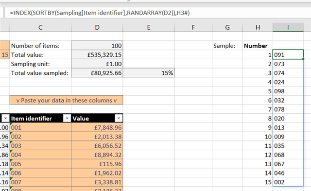
Our final function is:

=INDEX(SORTBY(Sampling[Item identifier],RANDARRAY(D2)),H3#)

We also want to pull the associated value for each item - we can easily do that using the new XLOOKUP function (which, if you’re using dynamic arrays, should also be available):

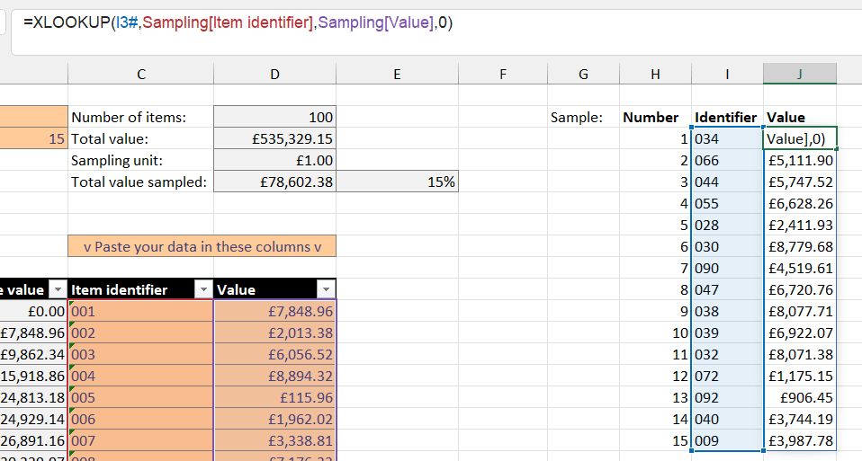
Once again we have used a #-reference to make a spilled function that will resize as the sample size chosen is changed.

Monetary unit sampling

If you're not familiar with monetary unit sampling, the idea is that, instead of considering each item individually, we consider each "pound" (or other unit) of the total value represented - so £1 is the first pound of the first item, and £7,849 is the first pound of the second item (in the above example), and so on. Instead of picking items, we pick random pounds within the range (from £1 to £535,329), which will mean that larger items are more likely to be chosen. However, we ignore any duplicates picked so that the total sample is still the desired size.

This is trickier to convert into a function, but it's still possible! Here's the process we will use:

1. List out all the "pounds" in the sample in order.
2. Sort the list into a random order.
3. Associate each pound in the list with the item it represents - larger items are statistically more likely to occur earlier in the list.
4. Remove all duplicates to create a 100-item list.
5. Pick the number of items needed to create the final sample.

Steps 1, 2, and 5 are essentially identical to the first process - except we will be using the total value of the sample as the list length instead of the number of items. Here's a look at where we are after steps 1 and 2:

The array spills down a full 500,000 rows! Our current work-in-progress formula is:

=SORTBY(SEQUENCE(D3/D4),RANDARRAY(D3/D4))*D4

Note that we divide the sizes of the sequences by the sampling unit, then multiply the resulting sequence by the unit again. This makes no difference in the case where the sampling unit is £1, but for populations where the total exceeds £1,000,000 it will prevent the array becoming too large and causing errors.

Next we need to convert these "pounds" into the items that contain them in our sorted list. While we might have used INDEX MATCH to do this previously, XLOOKUP can again take care of this to match the highest identifier that is less than or equal to the search value.

The formula is now (previous formula in bold):

=XLOOKUP(SORTBY(SEQUENCE(D3/D4),RANDARRAY(D3/D4))*D4,Sampling[Cumulative value],Sampling[Item identifier],,-1,1)

This list of course contains many duplicates. To remove them, we will use UNIQUE - and then finally we will pass our list to and INDEX as before. Here's the finished article:

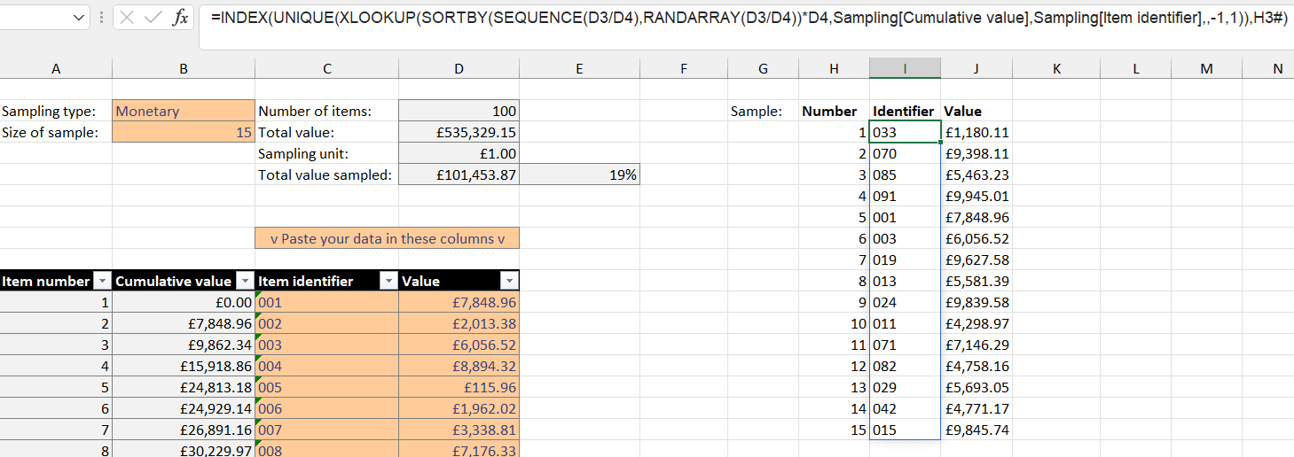
And the formula in its entirety:

=INDEX(UNIQUE(XLOOKUP(SORTBY(SEQUENCE(D3/D4),RANDARRAY(D3/D4))*D4, Sampling[Cumulative value],Sampling[Item identifier],,-1,1)),H3#)

This is obviously much more complex than the previous example, but it works in a very similar way. Now we have a sample that's weighted towards the larger items in the list.

Bringing it all together

Finally, combine our two sampling type formulas with an IF function, checking against the selected dropdown in cell B2, and you have a fully-functioning sampling tool:

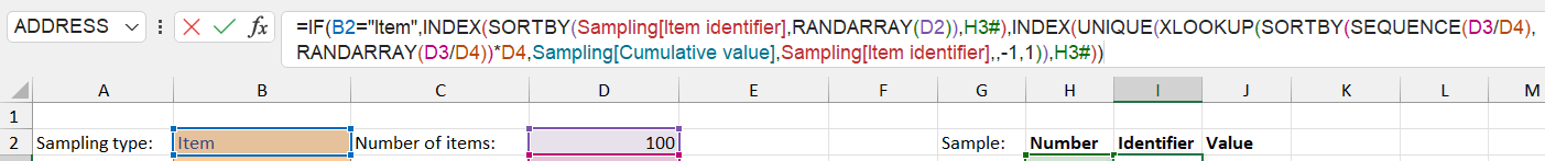
=IF(B2="Item",INDEX(SORTBY(Sampling[Item identifier],RANDARRAY(D2)),H3#),INDEX(UNIQUE(XLOOKUP(SORTBY(SEQUENCE(D3/D4),RANDARRAY(D3/D4))*D4,Sampling[Cumulative value],Sampling[Item identifier],,-1,1)),H3#))

One more thing – as this tool is formula driven, every change to the sheet will trigger the formulas to recalculate, and will therefore change the random sample. This can be overcome by either copying and Paste>Values for the generated sample, or by going to Formulas>Calculation Options and turning off the automatic calculation on the spreadsheet. Don’t forget to do this!

You can watch the video here that went with the original TOTW article:

(note that there are some changes to the formulas between the video and this revisited article)

Download the template yourself and have a go at using it - and try stepping through the calculations with Formulas => Evaluate Formula to see how the dynamic arrays work!

Related Posts

• Hooray for Arrays webinar
• TOTW #437 - Revisiting dynamic arrays
• Excel Tips and Tricks #443 - Next level FILTERing
• Excel how to: speed up entering formulae – Dynamic Array