Exploring Charts (Graphs) in Excel - Part 11: Adding Trendlines through data series and using the functions =FORECAST, =TREND, =SLOPE and =INTERCEPT

The financial services standard disclaimer is important to bear in mind ‘Past performance does not guarantee future results’.  Therefore, in creating forecasts extrapolated from past data can be a useful contributory factor, but obviously cannot be relied upon.

Trendlines

To illustrate some of the features and functions we will use the following data series with the aim of forecasting the final months of the year.

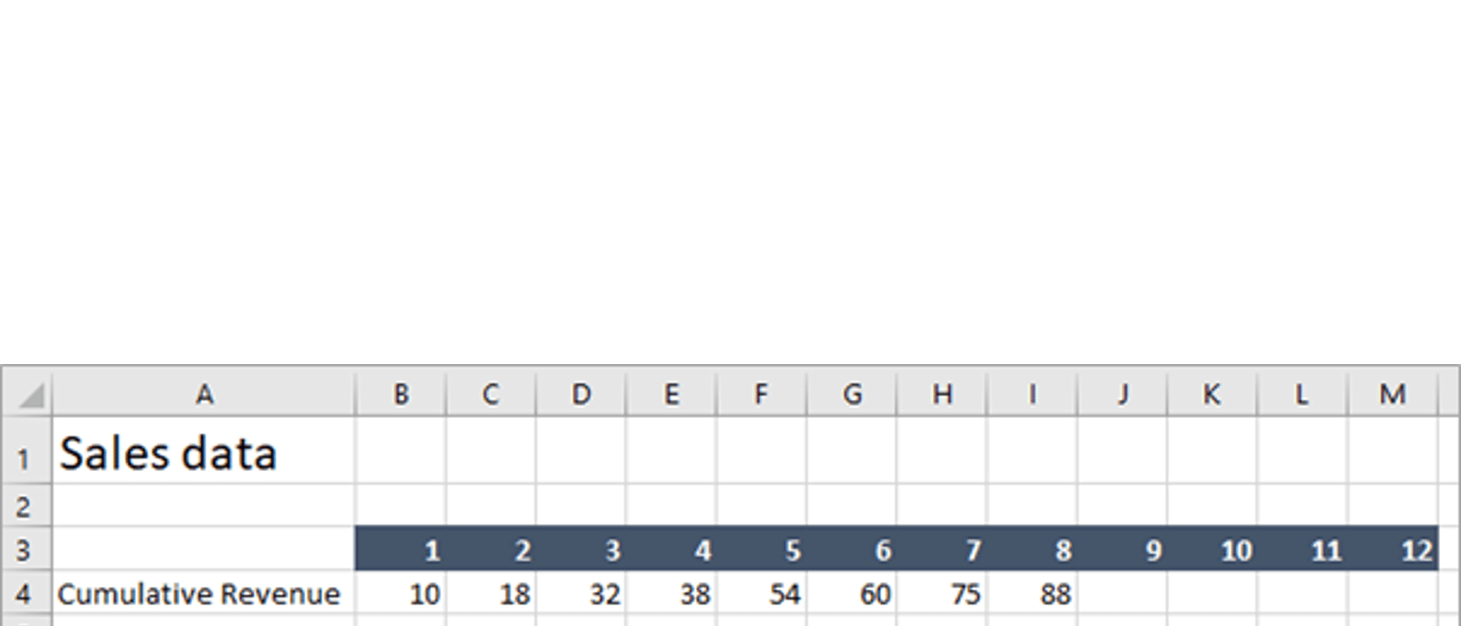
First plot the data on a 2D line chart (See Blog 3 for how to complete this).

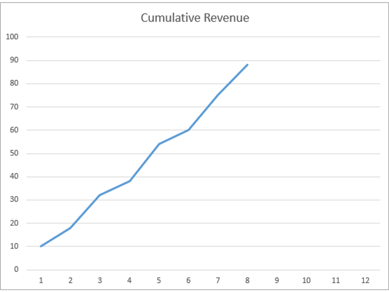
We can now add a Trendline to find ‘the line of best fit’ through the data.  Right click on the line and on the menu the option Add Trendline appears.

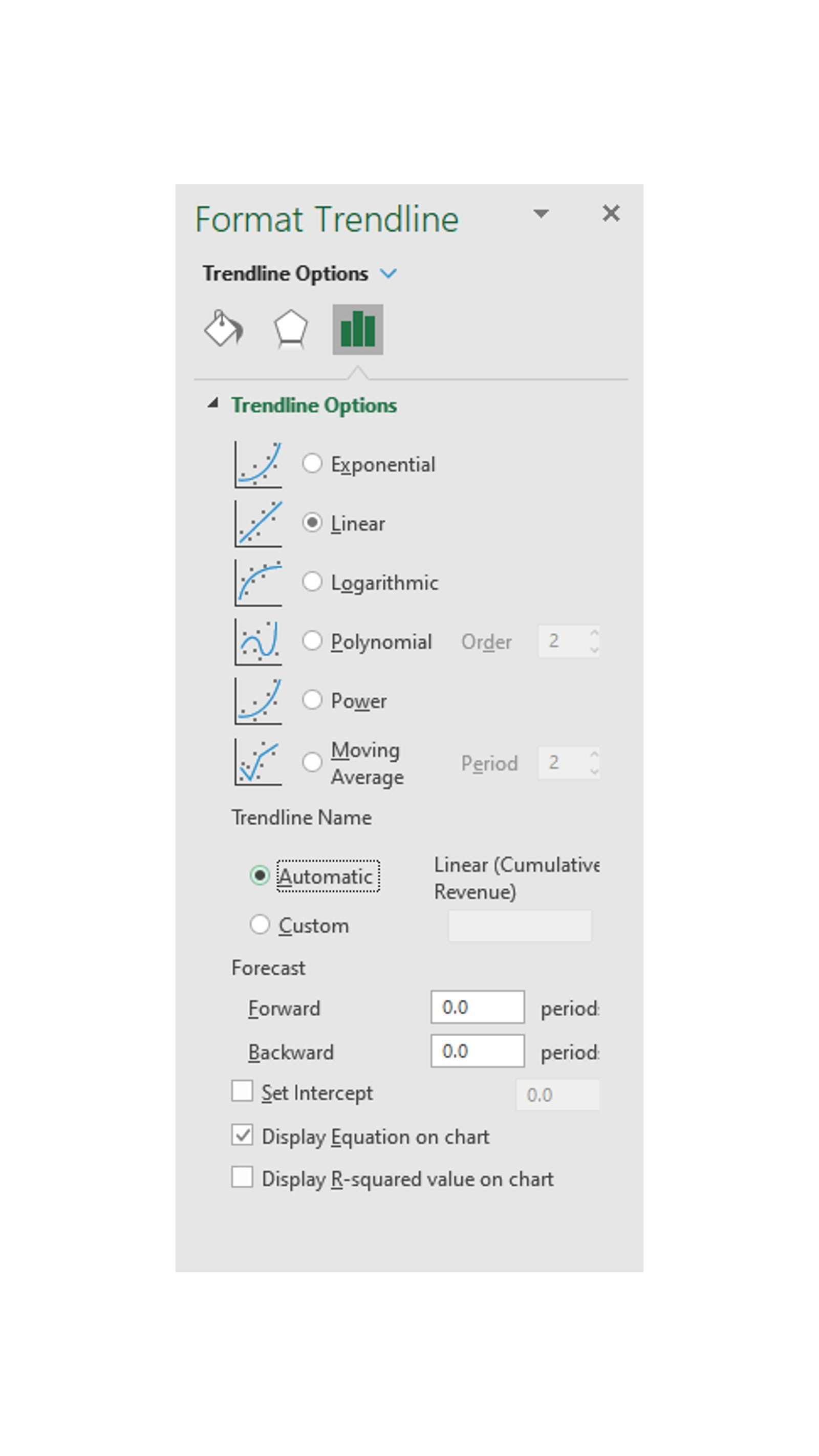
Several features are available.  First choose the profile of the data you want to trend.  We are using a simple Linear relationship in this example, but on the menu above you can see five other alternatives. For financial data the other option commonly used is Moving Average (see below).

The Linear Trendline uses least squared regression.  This is great for data that has an obvious trend.  If the data has outlying values these can distort the ‘line of best fit’ and produce a somewhat meaningless forecast.

In the Forecast options the number of Forward and Backward periods can be entered.  On the chart the X axis will be extended to display the extrapolated Trendline over these periods.

At the bottom of the dialog box there is an option to display the equation for the ‘line of best fit’ on the chart.

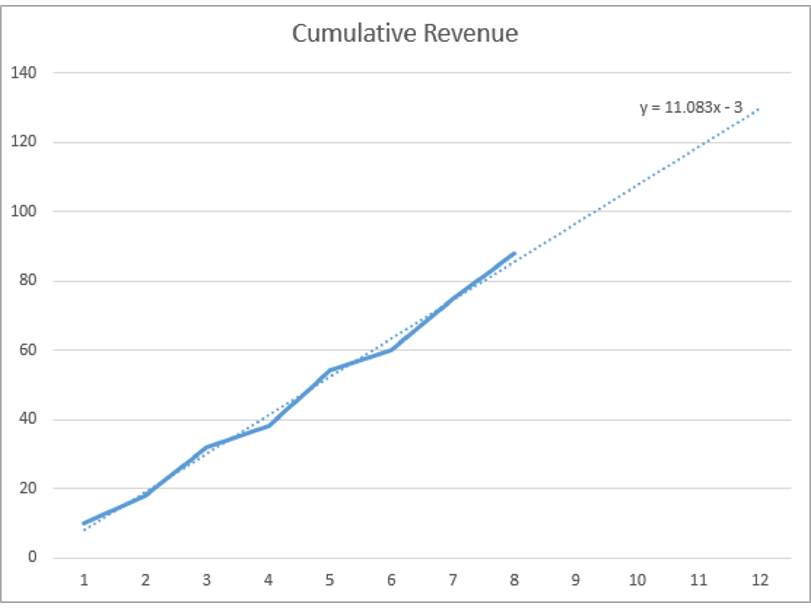
To extract the formula for the equation can be achieved with the following Excel functions:

The function =LINEST can also be used to derive both values in adjacent cells (the result spilling one cell to the right of where the formula is written).

Using this formula, we can derive a forecast for period 9:

(11.083 x 9) – 3 = 96.75

The forecast results can also be derived using two other functions:

Moving Averages

To use the Moving Average Trendline you will need monthly data rather than cumulative.

The same data set as above, but now displayed monthly would be as follows:

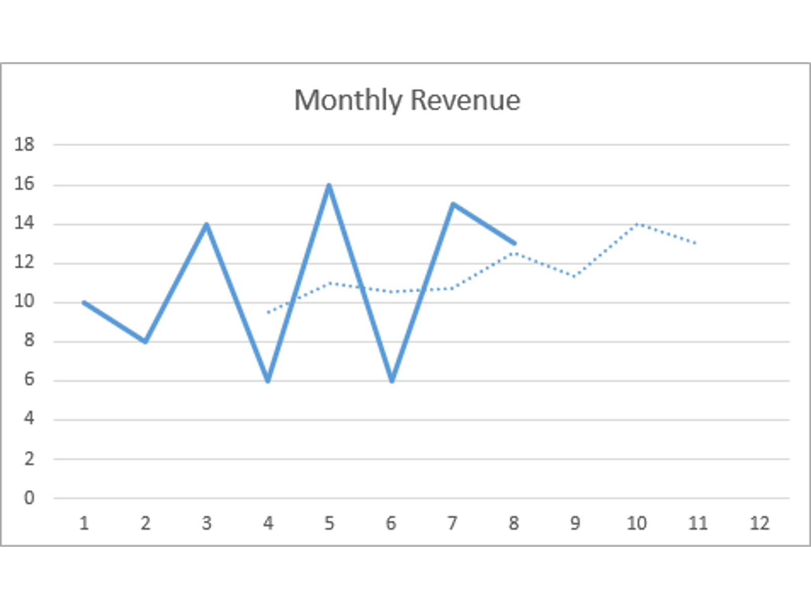
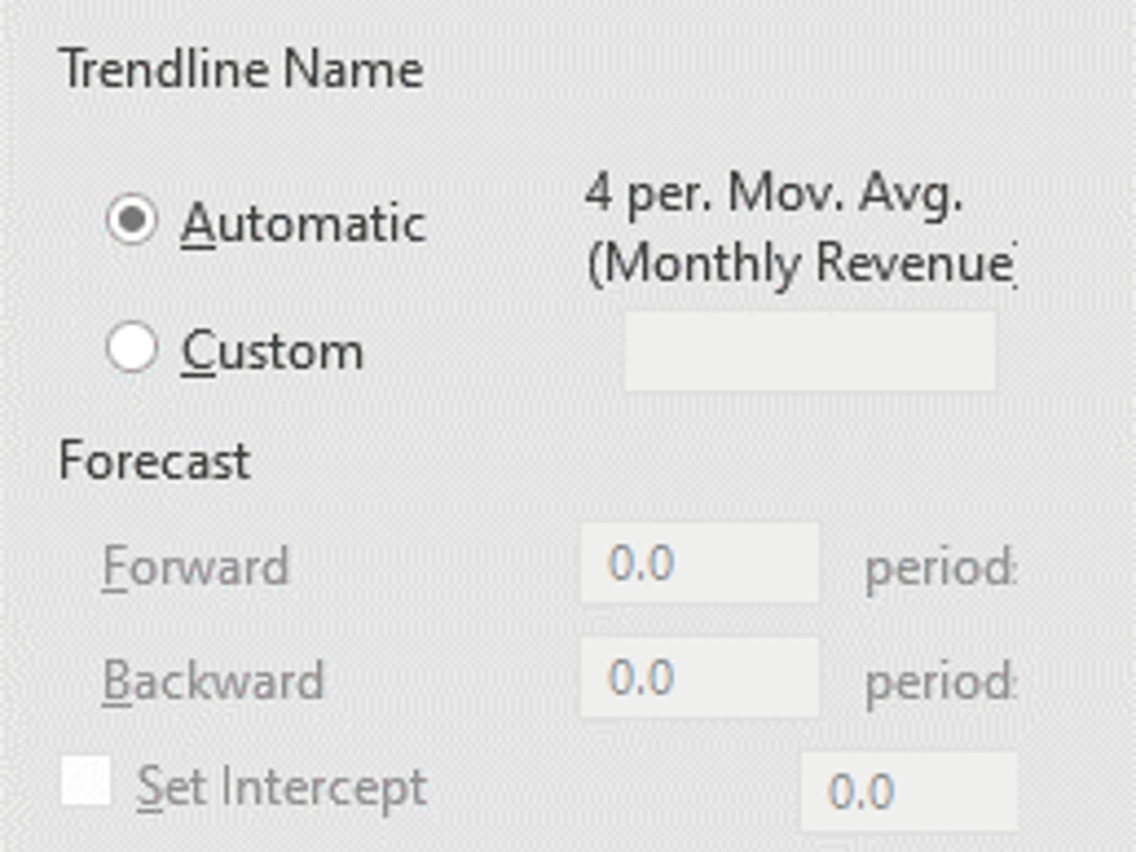
This Trendline using a four-period average (to smooth the peaks and troughs).  The default when the dialog box is first opened is set to two.  There is no equation available to show on the chart hence that area of the dialog box is greyed out.

Another way to derive moving average data that provides greater clarity on the values calculated and displayed is by using the Data Analysis function (this option has a host of other statistical data options too).

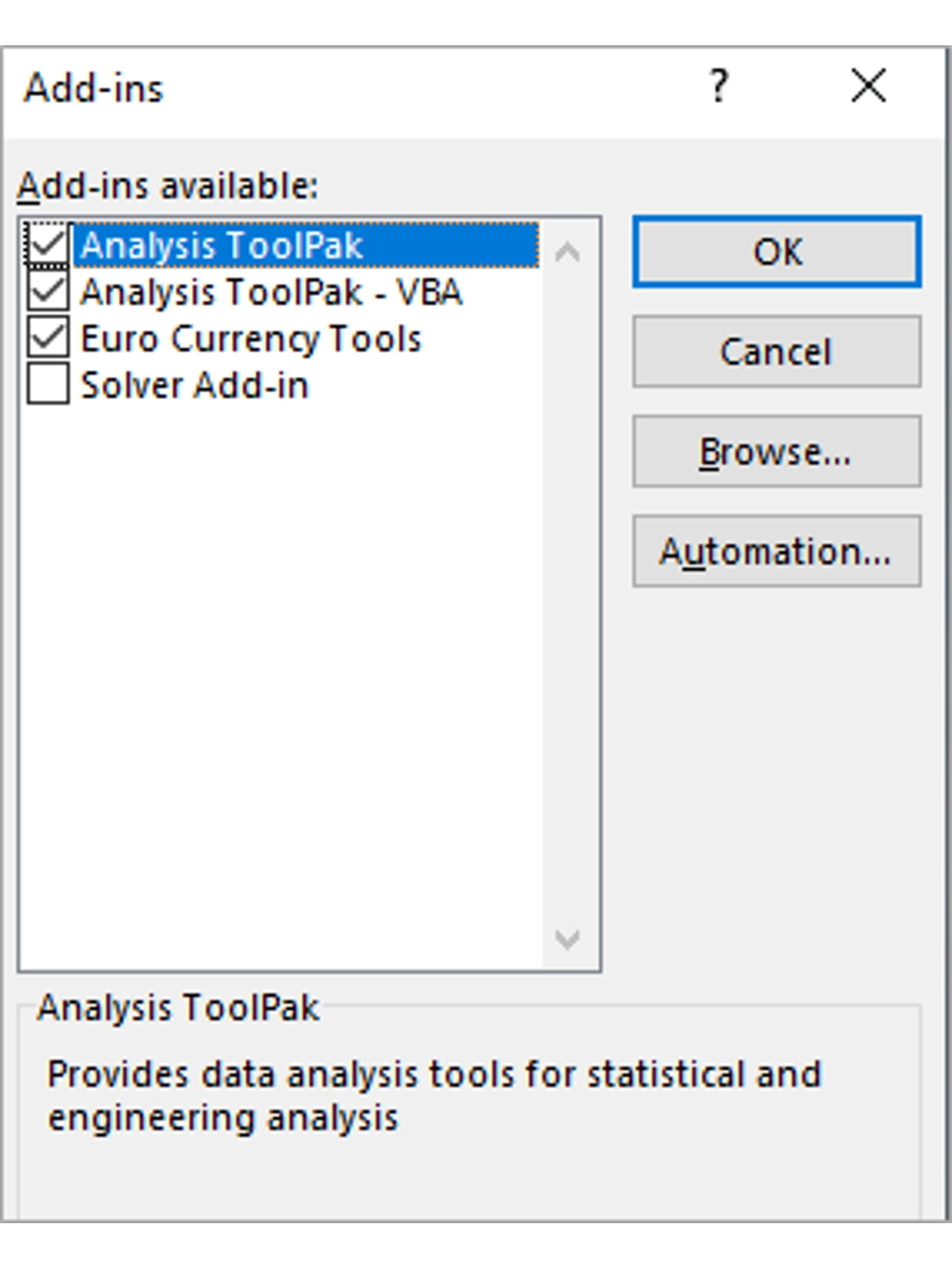
On the Data Ribbon there is a section called Data Analysis, but this is only available if the Analysis Toolpak has been enabled.

To enable the Analysis Toolpak go to the File Menu, select Options and select Add-ins.  At the bottom of this dialog box will be a section titled Manage: in the drop down select Excel Add-ins and press the button Go…  finally check the box for Analysis Toolpak.

Once opened from the right-hand side of the Data Ribbon the Moving Average calculation can be set up as follows:

The Input Range is the data, Interval is the 4-period calculation, and the Output Range is where the data is to be placed once calculated.

Don’t be put off by the # signs, it is in the first three periods as it has insufficient data to calculate a 4-period moving average for these months.  These points will not be displayed when plotted (more on this in the next blog).

In our final blog we will round off the series by covering a range of useful features including: controlling zeros and missing data, hanging lines using =NA, using conditions to highlight attributes (peaks, troughs), saving a chart as a picture to use in other applications.