
Hello and welcome back to Excel Tips and Tricks! This week have a Creator level post where we take a look at Excel functions that are harder to use with arrays or ranges.
We all love the new dynamic array functions in Excel. One function handles the entire range of cells we want to operate on and can return an array automatically resized to fit the size needed for the result. However, you may have been disappointed to find that you may have trouble getting some Excel functions to return arrays.
LOGICAL FUNCTIONS AND, OR
A logical condition is used in many functions such as IF and FILTER. For example, LEFT(A2:A200,1)="U" is a condition that tests whether each cell in the range A2:A200 begins with U.
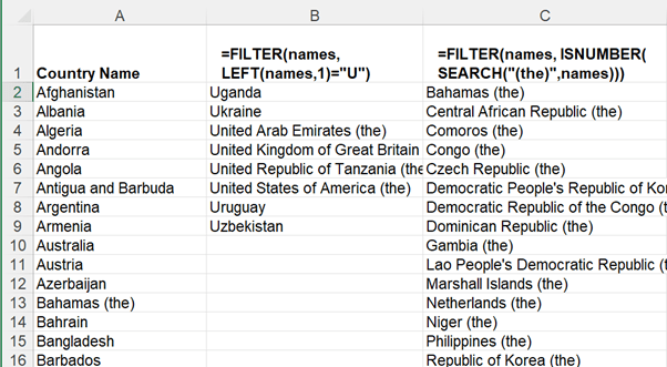
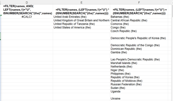
When you want to use multiple conditions in FILTER expressions, you might think first of using =FILTER(list, AND( condition1, condition2) ). The AND() function can accept an array and return a single TRUE value if all are true. For example, AND( {TRUE, TRUE, FALSE} ) will return FALSE. But AND does not return arrays. AND({TRUE,TRUE},{TRUE,FALSE}) returns only one result, FALSE, not the expected array {TRUE, FALSE}. The way to combine them to produce an array, where each element is true only when both elements of the two arrays are true, is to multiply the two tests. Multiplication returns a numeric result where 1=True, 0=False.
={TRUE,TRUE}*{TRUE,FALSE} returns {1,0}.
So, for AND we can use =FILTER(list, condition1 * condition2 ).
And for OR we can use =FILTER(list, condition1 + condition2 ).
Because multiplication has a higher priority than a logical test for equality, in most cases you will have to put brackets around the (condition) expression to force that to be evaluated first before the multiplication takes place. We will use the name 'list' for A2:A200.
For example, =FILTER(list,(LEFT(list,1)="U") * (RIGHT(list,1)="N") )
If you omit the prioritising brackets, you would get #VALUE! because Excel would first try to multiply the "U" by the TRUE or FALSE result of the RIGHT() expression.
EOMONTH() – DATE OF END OF MONTH
EOMONTH does not work when you pass in a range or a spilled array cell.
EOMONTH(A4:A8,0) and EOMONTH(A4#,0) both give #VALUE!
However, there is a workaround; convert the range to an array of values. Microsoft suggest using the VALUE function, e.g., EOMONTH( VALUE(A4#) ) but a simpler way is EOMONTH ( +A4# )
The DATE, YEAR, MONTH, and DAY functions all spill so instead of EOMONTH you could use: DATE(YEAR(D4#),MONTH(D4#)+1,0)
EDATE() - SHIFT DATE N MONTHS IN FUTURE OR PAST
This has the same behaviour as EOMONTH; if you pass in a range, =EDATE(B1:C1,1) it returns #VALUE!, if you pass in an array =EDATE(+B1:C1,1), it returns an array. So, it has the same workaround.
The same applies to NETWORKDAYS, WEEKNUM, WORKDAY, YEARFRAC, and many other functions.
Functions that can return a range reference are OFFSET, INDEX. XLOOKUP, CHOOSE, SWITCH, IF, IFS, INDIRECT.
Are there other functions you find difficult to get into array shape? Try the workarounds above and let us know if there are any that still resist arrayifying.
- Excel Tips and Tricks #506: Creating a single master list after merging data
- Excel Tips and Tricks #505 – 3 ways of converting US Dates into UK formats
- Excel Tips and Tricks #504 - Accessing accessibility checkers for good spreadsheet practice
- Excel Tips and Tricks #503 – Printing under pressure, super quick presentation tips
- Excel Tips and Tricks #502
Archive and Knowledge Base
This archive of Excel Community content from the ION platform will allow you to read the content of the articles but the functionality on the pages is limited. The ION search box, tags and navigation buttons on the archived pages will not work. Pages will load more slowly than a live website. You may be able to follow links to other articles but if this does not work, please return to the archive search. You can also search our Knowledge Base for access to all articles, new and archived, organised by topic.